The Eigenprinciple

Part A · Foundation

Chapter 1

The Tuning Fork and the Rule for Next Time

A struck tuning fork emits a single, almost pure tone, and it does so reliably enough that for two centuries it served as the reference standard for tuning instruments. What is remarkable is not the tone itself but its stability: whether the fork is struck gently or hard, whether warm or cold, the frequency stays the same. This behaviour suggests that the system prefers a particular vibration pattern and returns to it after every disturbance.

The following develops where this stability comes from. The answer is a pattern that runs through the entire post and is called here the eigenprinciple: a system that follows a simple local rule develops, on its own, characteristic and stable patterns. These patterns are not an external prescription but a mathematical consequence of the rule.

A rule for next time

A point on the vibrating prong can be described completely by two quantities. Let \(x\) be the displacement of this point from its rest position and \(v\) its velocity. The elasticity of the material determines how these two quantities change from one small time step \(\Delta t\) to the next:

The first rule describes, intuitively, pure motion: whoever moves with a given velocity is, after one time step, further along by the product of velocity and time step. The second rule describes, intuitively, the restoring force of the material: the further the point is displaced, the more strongly it is pulled back towards rest. Here the constant \(k/m\) – stiffness divided by mass – determines how vigorous this restoring is.

The entire behaviour of the tuning fork follows from these two lines. Applied many thousands of times in succession, they produce not an arbitrary curve but a pure sine oscillation, and that independently of the initial displacement. The following display carries out this iteration step by step.

The closed ellipse in phase space is the heart of the matter. It means, intuitively, that the system returns to its initial state after every full cycle; precisely this recurrence makes the tone stable. Mathematically the update rule is a linear map, and the oscillation is its eigenpattern. This means that the stability of the tuning fork and the notion of an eigenvector are two descriptions of the same fact – a connection developed in the next chapter.

Part A · Foundation

Chapter 2

What an Eigenvector Really Is

A matrix is a linear map: vector in, vector out. Most vectors change both their length and their direction in the process. A few vectors, however, keep their direction and are merely stretched or compressed. These direction-preserving vectors are called eigenvectors, the associated stretching factor is the eigenvalue.

How the eigendirections are found

We seek vectors \(\mathbf{v}\) for which the map \(A\) merely produces a stretch, that is \(A\mathbf{v} = \lambda\,\mathbf{v}\) with a scalar \(\lambda\). This equation means, intuitively, that input and output lie on the same line through the origin. Rewritten as \((A - \lambda I)\,\mathbf{v} = \mathbf{0}\), it has a non-trivial solution exactly when the determinant \(\det(A - \lambda I)\) vanishes.

This determinant is a polynomial in \(\lambda\), the characteristic polynomial. Its roots are the eigenvalues, and to each eigenvalue belongs an eigendirection. Here a real map need not possess real eigenvalues: a rotation displaces every vector, so that none stays direction-true – the visualization above shows this case under the preset Rotation.

This closes the arc back to Chapter 1. The update rule of the tuning fork was a linear map, applied at every time step; the stable oscillation corresponded to its eigendirection, and the frequency was fixed by the associated eigenvalue. This means that eigenvectors are not an algebraic curiosity but describe which patterns a repeatedly applied process prefers.

Part A · Foundation

Chapter 3

From Vectors to Functions: the Eigenfunction

The same idea carries over when a whole function takes the place of the vector. An eigenfunction is a function that, under an operation – say the second derivative or the Fourier transform – keeps its shape and is only scaled by a factor. This definition transfers the notion of an eigenvector from finite vectors to the infinite-dimensional space of functions.

Standing waves on a plate

A clamped plate cannot vibrate arbitrarily. It takes on only certain patterns, the eigenmodes, in which certain lines stay permanently at rest. Scatter sand on the plate and it gathers along these nodal lines, making the pattern visible; Ernst Chladni demonstrated these figures from 1787 onward.

Only integer mode numbers are allowed. This discretisation is no accident but follows from the boundary conditions: the plate is fixed at its edge, and only patterns with an integer wavenumber satisfy that condition. The same quantisation produces the discrete energy levels of an atom; Schrödinger therefore titled his 1926 paper Quantization as an Eigenvalue Problem.

Every curve as a sum of eigenfunctions

For the vibrating string the eigenfunctions are the sine modes. Here a property holds that carries far beyond the string: every sufficiently smooth function can be written as a sum of these sine eigenfunctions, \(f(x) = \sum_n c_n \sin(n\pi x)\). This sum means, intuitively, that the eigenfunctions form a complete basis – just as every vector is assembled from basis vectors.

That complete eigenfunction bases exist at all is the content of Sturm-Liouville theory from 1836. It shows that a broad class of physical differential equations possesses a complete, orthogonal system of eigenfunctions; the particular boundary condition selects which one. Hence sine functions appear for the string, Bessel functions for cylindrical symmetry, and Hermite functions for the quantum-mechanical oscillator. This means that decomposing into eigenfunctions is not a special trick of individual fields but the common structure behind acoustics, heat conduction and quantum mechanics.

Part B · Applications

Chapter 4

Faces in the Data Stream: Principal Components

So far eigenvectors were a property of a given map. In data analysis the direction of view reverses: from the data themselves a matrix is built, whose eigenvectors reveal the inner structure of the data. This procedure is Principal Component Analysis (PCA).

The axes of greatest spread

Let a cloud of data points be given. From it the covariance matrix is computed, whose entries describe how strongly the coordinates vary together. The eigenvectors of this matrix mean, intuitively, the directions along which the data spread most; the associated eigenvalue states how large that spread is. The first principal axis thus captures the largest part of the information, the second the next largest, and so on.

Herein lies the practical benefit: if the first axis carries most of the spread, the second can be neglected without losing much information. High-dimensional data are thus compressed onto a few axes. This means that PCA is a compression whose basis is not prescribed but obtained from the data as their eigenstructure.

Eigenfaces

If face images are taken as data points – each pixel a coordinate – the principal axes yield the eigenfaces. Matthew Turk and Alex Pentland showed in 1991 that every face can be represented as a mean face plus a weighted sum of a few eigenfaces. A few dozen coefficients suffice to recognise a face.

The same idea carries the deepfakes post: there an autoencoder replaces linear PCA with a non-linear generalisation, yet the principle remains that a face is described by a few coordinates in a learned basis. This means that face recognition solves, at its core, the same eigenvalue problem as the vibrating tuning fork – only that the eigenvectors here come from data rather than from an equation of motion.

Part B · Applications

Chapter 5

The Web as a Random Process: Markov and PageRank

A Markov chain describes transitions between states in which the current state alone decides the next. The probabilities of these transitions form a matrix. Let an initial distribution over the states be given, then multiplication by this matrix yields the distribution one step later.

The distribution that no longer changes

If this step is repeated, the distribution converges under mild conditions to a fixed vector, the stationary distribution. This vector no longer changes under the transition matrix; it therefore satisfies \(\boldsymbol{\pi} P = \boldsymbol{\pi}\) and is thus the eigenvector for eigenvalue one. The Perron-Frobenius theorem guarantees that for a stochastic matrix this eigenvalue exists, is largest in magnitude, and is simple.

PageRank: the web as a Markov chain

Google's original ranking algorithm treats the web as a Markov chain. The states are web pages, the transitions are the links. An imagined visitor follows, with probability \(d\), a random link of the current page and jumps, with probability \(1-d\), to an arbitrary page of the web. This damping factor \(d\), usually \(0.85\), prevents the visitor from getting stuck in link-free dead ends.

The PageRank of a page is its visit frequency in the stationary state – again the dominant eigenvector, this time of the so-called Google matrix. Here the damping factor acts as a regularisation that makes the problem stable and uniquely solvable. The eigenvalues post shows that this damping factor corresponds structurally to the same term as the regularisation parameter of ridge regression. This means that stabilising a web search and avoiding overfitting in machine learning are two manifestations of the same intervention into an eigenvalue spectrum.

Part B · Applications

Chapter 6

When Bridges Dance: Resonance

So far the eigenpatterns were desirable or useful. This chapter shows their dangerous side. Every mechanical structure possesses eigenfrequencies, that is, vibration patterns it preferentially takes on. These eigenfrequencies are the eigenvalues of the structure's equation of motion. When a periodic excitation meets one of these frequencies, it transfers its energy especially effectively, and the motion builds up – a process called resonance.

Tacoma Narrows, 1940

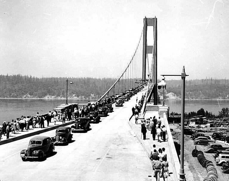
A few months after its opening, the Tacoma Narrows Bridge entered a self-amplifying torsional oscillation in moderate wind and collapsed. The wind supplied no periodic excitation in the simple sense; rather, vortices shed rhythmically from the deck, their frequency close to an eigenfrequency of the bridge. This mechanism – aeroelastic flutter – has since been a fixed part of bridge engineering.

Millennium Bridge, 2000

On the opening day of the London Millennium Bridge, it began to sway sideways under the weight of pedestrians. Here no external excitation acted but a feedback: a small sideways motion led those walking to adjust their step unconsciously to the sway, which amplified the motion and drew in further people. This transition from disordered to synchronised walking is an example of synchronisation, described by the Kuramoto model.

Both cases share the same cause. A system with pronounced eigenmodes is excited near an eigenfrequency and responds with growing amplitude. This means that the stability of the tuning fork's tone and the collapse of a bridge are two sides of the same coin: in the one case the preferred eigenpattern is desirable, in the other destructive.

Part B · Applications

Chapter 7

The Bell Curve as a Preferred Shape

When many independent random influences are summed, the same distribution almost always results: the bell curve. The Central Limit Theorem describes this observation precisely. At first glance it does not belong in this chapter, for there is no talk of eigenvalues here. On closer inspection, however, the same pattern carries.

The mathematical operation that combines two independent random influences is the convolution of their distributions. The Central Limit Theorem states, intuitively, that the repeated convolution of arbitrary distributions tends towards a single shape: the Gaussian bell curve. This shape no longer changes its form under further convolution, only its width.

Thus the bell curve is a fixed point of convolution – and a fixed point is nothing other than an eigenvector for eigenvalue one, here in the space of probability distributions. This means that the ubiquity of the normal distribution has the same cause as the stability of the tuning fork's tone: it is the preferred, self-reproducing pattern of a repeatedly applied process.

Part B · Applications

Chapter 8

The Recurring K: Quantum and AI

The preceding chapters sought the eigenprinciple in mechanics, data analysis and probability theory. This chapter leads it back to where the earlier posts of this blog have already met it: into quantum mechanics and machine learning.

In quantum mechanics the propagator describes how a particle evolves from one place to another. It is written as a sum over eigenstates, weighted by phase factors of the energy eigenvalues:

In kernel methods of machine learning the kernel describes how similar two data points are. It too is written as a sum over eigenfunctions, weighted by their eigenvalues:

Both expressions carry the same letter \(K\), and that is no coincidence. Both are a spectral decomposition: a sum over eigenfunctions, each weighted by its eigenvalue. This means, intuitively, that the question How does a quantum particle get from A to B? and the question How similar are two data points? have the same mathematical form.

The same structure reaches into modern language models. The attention mechanism of a transformer computes weighted similarities between tokens and can be read as a kernel operation whose behaviour is governed by an eigenvalue spectrum. How this spectrum changes when a model grows is the subject of the post on emergence.

Part C · What it says about nature

Chapter 9

Discovered or Invented?

The preceding chapters met the same structure in very different fields. This recurrence can be read in two ways. On the first reading we merely project a familiar mathematical tool onto everything we examine; the eigenstructure would then lie in our gaze, not in the things. On the second reading the eigenstructure is a feature of reality itself, which we discover.

One argument speaks for the second reading. The eigenpatterns appear in physics, biology and computer science independently of one another, derived from entirely different starting assumptions. Were they mere projection, they would have to break at the points where the fields do not know each other. Instead they deliver the same structures there. This finding can be read cautiously in the sense of a spectral realism: the eigenstructures are not invented but found.

Caution is nevertheless warranted, and let the assumption be named openly here. That a tool fits everywhere may also mean that it is coarse enough to fit everywhere. Linear maps are the simplest non-trivial class of maps, and eigenvalues are their natural vocabulary. Part of the ubiquity is therefore likely due to the simplicity of the tool, not to a depth of nature alone. A final decision between the two readings is not claimed here.

Stability as selection

One connecting thought remains regardless of this question. Through all chapters ran the same principle: stable patterns remain, unstable ones cancel out. The tuning fork returns to its eigenpattern; the stationary distribution is the state that reproduces itself; the bell curve is the shape preserved under convolution. In each case the eigenpattern is not what begins loudest, but what endures.

The same selection principle carries two earlier posts of this blog. In the quantum post, those paths survive whose phases add constructively, while the rest cancel through destructive interference. In the post on God as an emergent phenomenon, coherent configurations prevail as attractors of a dynamic. This means that eigenpatterns, stable quantum paths and coherent world-views are descriptions of the same process: a process is applied repeatedly, and what survives it unchanged remains.

Herein lies the glass bead game of this blog. Not in the claim that everything is the same, but in the more precise observation that very different objects share the same mathematical core. Erwin Schrödinger titled his 1926 paper Quantization as an Eigenvalue Problem. The line pursued here adds only that not quantisation alone, but a whole series of stable orders can be written as an eigenvalue problem – and that these orders arise because a process selects its own preferred patterns.

Frequently Asked Questions

What is the eigenprinciple?

The eigenprinciple is the observation that a system following a simple local rule develops, on its own, characteristic stable patterns – the eigenpatterns. These patterns are not an external prescription but a mathematical consequence of the rule, and are described by eigenvalues and eigenvectors.

What is the difference between an eigenvector and an eigenfunction?

An eigenvector keeps its direction under a matrix and is only stretched. An eigenfunction keeps its shape under an operation such as differentiation or the Fourier transform and is only scaled. It is the same idea, once in the finite-dimensional space of vectors, once in the infinite-dimensional space of functions.

What do PageRank and Principal Component Analysis have in common?

Both compute a dominant eigenvector. PageRank finds the eigenvector of the Google matrix – the stationary distribution of a random surfer. Principal Component Analysis finds the eigenvectors of the covariance matrix – the directions of greatest spread in the data.

Why does the same mathematics appear in such different fields?

Because stable patterns are exactly what a repeatedly applied process selects: stable structures persist, unstable ones cancel out. This selection principle leads, in mechanics, data analysis, probability theory and quantum mechanics, to the same eigenvalue structure.