Prefer watching over reading?
7 minutes · The double-slit experiment visually explained
Chapter 1
Waves, Arrows and the Double-Slit Wonder
A Stone, a Pond, a Puzzle
Throw a stone into a still pond. You know what happens: circular waves spread out, smooth, predictable, boring. Now throw two stones at the same time into different spots. Now it gets interesting. The waves from the two stones travel toward each other, and where they meet, something peculiar happens. In some places the water gets especially agitated – higher, wilder than from either stone alone. In other places, sometimes just a few centimeters away, there is a strange calm.
This phenomenon has a name: interference. And it is the most harmless, everyday thing in the world. Where the crest of one wave meets the crest of another, the heights add up – the water surges especially high. But where a crest meets a trough, they cancel each other out. Plus and minus, zero, silence.
So far, so reassuring. Now let us observe the same effect with light. And then the world gets strange.

Thomas Young and the Wall with Two Slits
In 1801, the English physician and polymath Thomas Young performed an experiment that is simple enough to recreate on a kitchen table, yet so profound that physics is still grappling with it two hundred years later.
The idea: take a light source. Place a wall in front of it with two narrow, parallel slits cut into it. Behind it, a white screen. If light were made of particles – tiny pellets flying in straight lines like bullets – you would expect two bright strips, directly behind the two slits.
But that is not what Young sees. And in two different ways.
First, the light fans out behind each slit. It doesn't fly straight through like a bullet through a hole – it spreads out in all directions, as if each slit were itself a new, tiny light source. This fanning out is called diffraction.
Aside · Why a single slit is enough
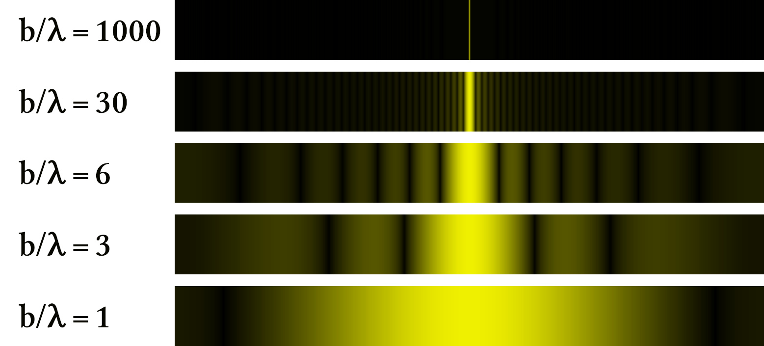
In the ideal thought experiment, slits are infinitely narrow – mathematical points. In reality, every slit has a finite width. And that width has consequences.
Think of the slit not as a single point but as a row of points, tightly packed side by side. Each of these points within the slit opening acts like its own tiny light source, radiating in all directions. All these tiny sources overlap – and because they sit at slightly different positions within the slit, their contributions travel slightly different path lengths before reaching the screen.
Straight ahead, directly behind the slit, all contributions arrive almost simultaneously – they reinforce each other. But at an angle, the paths from different points within the slit have different lengths. Some contributions cancel out, others reinforce. The result: even a single slit produces a pattern – a broad bright strip in the center and weaker strips on either side. And – counterintuitively – the narrower the slit, the wider the light fans out.
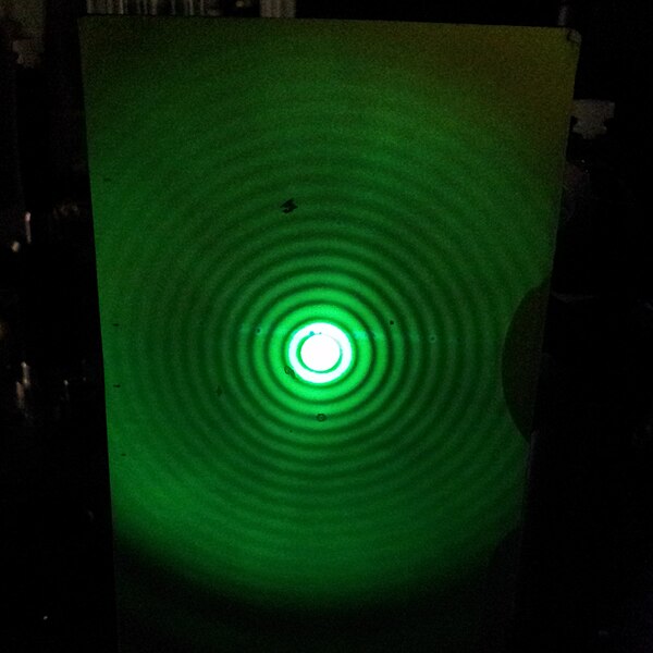
What you see here is not a double-slit effect. It is a single-slit effect – or, for the circular aperture, a single-hole effect. Interference does not need a second slit. It only needs an opening that is not infinitely narrow – and the fact that contributions from different points within that opening can overlap.
Later, when we learn Feynman's arrow method, it will become clear: this single-slit pattern is nothing but adding arrows – over all paths through the opening. The physics behind diffraction and interference is one and the same.
But the crucial thing about the double slit only arrives with the second slit. Because now there are two such fanning-out light sources, close together. And where their contributions overlap, something happens that diffraction alone cannot explain: in some places they reinforce each other, in others they cancel out. The result is a pattern of many bright and dark fringes, alternating, spread across the entire screen. Bright, dark, bright, dark. Interference.
Diffraction and interference – Richard Feynman later said that nobody ever managed to define the difference between the two satisfactorily. Fundamentally it is the same phenomenon: contributions from different directions overlap and either reinforce or cancel. With one slit we call it diffraction, with two we call it interference. The physics behind it is identical – and later, when we learn Feynman's arrow method, we will see that both are nothing but adding arrows.
For Young, at any rate, the case was clear: light is a wave. Debate over, Newton was wrong, Huygens was right.
Then came the electrons.

The Experiment Nobody Understands
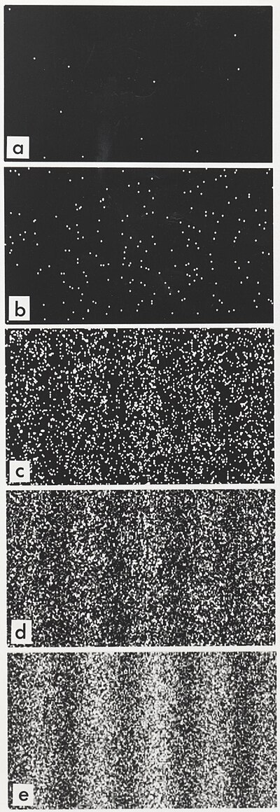
Electrons are particles. Tiny things with mass and charge. They bounce off walls, they get deflected by magnets, you can count them, one by one. An electron is an electron, not half of one, not some diffuse something. If you place an electron detector behind the double slit, you hear click. One click, one electron. Not a hiss, not a swoosh. Click.
So: two slits. Fire electrons one at a time. One after another. The first hundred hits look random. But after tens of thousands of clicks, a picture forms: fringes. Bright, dark, bright, dark. Interference. Just like the water waves.
Stop. Wait.
The electrons were fired one at a time. There was only ever a single one in flight. What could it have interfered with? With itself?
Maybe each electron goes through one particular slit, and we just don't know which? Good idea. Wrong. Because when you install a detector at the slits that determines which slit the electron went through – the interference pattern vanishes. Instantly. Completely.
The electron seems to know whether you are watching. At this point most popular-science accounts veer into philosophy. Consciousness of the observer, collapsing wave functions, cats in boxes. All of that is either wrong or at least unhelpful. What actually helps is an arrow.
The Arrow That Explains Everything
Forget for a moment everything you have ever heard about quantum mechanics. We start from scratch. And the only thing we need is a little arrow.
Imagine a clock. An analog one, with a hand. This hand rotates, steadily, in a circle. It has a certain length and points in a certain direction at every moment. That is all. Length and direction.
In quantum mechanics, every process a particle can carry out – "fly from here to there" – gets assigned such an arrow. Not a probability, not yes or no, but an arrow with length and direction. Physicists call this arrow an amplitude. And there is exactly one rule to turn it into a probability: take the length of the arrow and square it. An arrow of length 0.3 gives a probability of 0.09. An arrow of length 0.5 gives 0.25. That simple.
But the magic is not in the squaring. The magic is in what happens when there are multiple possibilities.
Adding Arrows – and Suddenly Everything Changes
Back to the double slit. An electron flies from the source to the detector. There are two paths: through the left slit or through the right. Each path has its own arrow.
Now comes the rule that changes everything: when there are multiple possibilities leading to the same outcome, you add the arrows. Not the probabilities – the arrows. Lay them tip to tail. The resulting arrow – that is your answer. Then you square its length.
When the two arrows point in roughly the same direction: long resultant arrow, high probability. Bright fringe. When they point in opposite directions: short resultant arrow, no probability. Dark fringe.
That is interference. Not of waves in space, not of mysterious superpositions – but of arrows that add up.
And how does the arrow know which direction to point? That depends on the path. A longer path rotates the arrow further than a shorter one. More precisely: the arrow rotates in proportion to the path length. If the path through the left slit yields exactly one half rotation more than the path through the right slit, then the two arrows point in opposite directions. Cancellation. Darkness. If the path difference yields one full rotation, both arrows point the same way again. Reinforcement. Brightness. Bright, dark, bright, dark – the interference pattern falls out of the arrows like a transfer decal.
Why Looking Destroys Everything
When you set up a detector that determines which slit the electron went through, there are no longer any alternatives. In each individual case there is only one arrow, not two that could be added.
No adding of arrows, no interference. The electron does not "know" whether you are watching. It is not mysticism. It is bookkeeping. When two paths are indistinguishable, you add the arrows. When you make them distinguishable, there is only one arrow per trial. The addition drops out. The interference disappears.
What you now have in hand: We have not written a single integral, not used any complex numbers. All we said was: every path has an arrow. Multiple paths to the same destination? Add the arrows. Then square. And from that, the entire physics of interference fell out.
These arrows – these amplitudes – are the real core of quantum mechanics. Not the wave function (that is just a particular representation of the arrows). Not the Schrödinger equation (that just describes how the arrows rotate over time). The arrows are the foundation.
Try it yourself
You see the double-slit experiment as an interactive visualization. Drag the yellow dot on the screen to test different detector positions. Turn the sliders for slit separation and wavelength. And then: switch on the detector and watch the interference pattern disappear.
What you just saw: Two paths, two arrows, one addition. When the arrows point in the same direction (blue and purple nearly parallel), they reinforce each other – bright fringe. When they oppose each other, they cancel out – dark fringe. Switch on the detector, and there is only one arrow per trial. No addition, no interference.
But think further. What happens if you cut not two slits into the wall but three? Then there are three paths, three arrows. Five slits? Five arrows. And if there is no wall at all – how many paths are there? Infinitely many. The straight path. The path that takes a little detour. The path that first flies to the moon and comes back. The spaghetti-tangle path. Each of these paths has an arrow. And quantum mechanics says: add them all.
That sounds insane. It sounds impossible to calculate. And it sounds like the result would be utter chaos.
But the opposite is the case. Out of this apparent chaos, order emerges – and precisely the order we observe in everyday life. A thrown ball follows a parabola. A planet orbits the sun on an ellipse. Newton's laws. Classical physics. They are all hiding inside the sum over infinitely many arrows.
How that works is what we will figure out now.
Chapter 2
Two Rules That Generate the Entire Quantum World
In Chapter 1 we sent an electron through two slits. Each slit gave the electron an arrow. The two arrows were added: lay them tip to tail, measure the resultant, square – done, there was the probability. From that, the entire interference pattern fell out. At the end stood the question: if an electron "takes both slits at once" – does it perhaps take all conceivable paths at once?
The answer is yes. And the road there leads through two rules that are simple enough to fit on a napkin – and powerful enough that all of quantum mechanics follows from them.
The Rules
Richard Feynman reduced quantum mechanics to two instructions. Not two equations – two instructions for what to do with arrows.
Rule 1 – Alternatives: Add the arrows.
If a particle can get from A to B by multiple paths, and you don't know (and in principle cannot determine) which path it took – then every path gets an arrow, and you lay them tip to tail. The resultant arrow determines the probability.
Rule 2 – In sequence: Multiply the arrows.
If a particle first goes from A to B and then from B to C, then each leg gets an arrow. The arrows are multiplied: the lengths are multiplied, and the angles are added.
That's it. Two rules. No ifs, no buts.
What "Multiplying" Means
Multiplying arrows sounds abstract, but it is just as intuitive as the adding from Chapter 1.
Adding meant: lay them tip to tail. The resultant arrow goes from the start of the first to the end of the last.
Multiplying means: multiply the lengths, add the angles. If the first arrow has length 0.8 and is rotated by 30°, and the second has length 0.5 and is rotated by 45°, then the product has length 0.4 and is rotated by 75°.
Same Bookkeeping, Different Currency
You might be wondering: why arrows? Why not simply probabilities, as in ordinary physics? The answer is the key to everything that follows. And the best way to see it is through a concrete example.
The classical decision tree. Imagine electrons were bullets. A bullet flies at the wall with two slits. It goes through the left slit with 50% probability and through the right with 50%. Behind each slit it gets deflected – say, with 30% probability straight ahead and 20% slightly to the left. What is the probability of the bullet arriving at a particular spot on the screen?
In sequence → multiply: the probability for "left slit, then straight ahead" is \(0{,}5 \times 0{,}3 = 0{,}15\).
In sequence → multiply: the probability for "right slit, then straight ahead" is also \(0{,}5 \times 0{,}3 = 0{,}15\).
Alternatives → add: both paths lead to the same spot, so \(0{,}15 + 0{,}15 = 0{,}30\).
So far, so familiar. This is exactly how every decision tree you know from school or university works. And the result is predictable: probabilities are always positive. When you add two positive numbers, the result always gets bigger. More paths mean more probability. No path can "cancel" another. The pattern on the screen: two broad humps, one behind each slit. No fringes. No surprises.
The quantum decision tree. Now the same thing with arrows. Exactly the same rules – multiply for in-sequence, add for alternatives. But instead of the number 0.5, each slit has an arrow of length 0.5 pointing in a particular direction. And instead of 0.3, the next step has an arrow of length 0.3 with a different angle.
In sequence → multiply: multiply the lengths, add the angles. The result for the path through the left slit is an arrow of length 0.15 – so far identical. Likewise for the right slit: also an arrow of length 0.15.
But now: alternatives → add. And here something happens that is impossible with probabilities. The two arrows have different directions – because the paths through the different slits have different lengths and the arrow has rotated further along the way. When the two arrows point in similar directions: large resultant arrow. Bright fringe. When they point in opposite directions: the arrows cancel. Resultant arrow nearly zero. Dark fringe.
More paths can mean less probability. That is the sentence that separates all of quantum mechanics from all of classical physics. And it follows not from a new rule – the rules are identical. It follows from the fact that nature does not compute with numbers but with arrows.

The difference in one sentence: In classical physics you compute with probabilities (positive numbers that never cancel). In quantum mechanics you compute with amplitudes (arrows that can cancel each other). The bookkeeping rules are the same. Only the currency is different.
The Double Slit as a Special Case
An electron flies from source A through a wall with two slits to detector C. There are two possibilities: through the left slit (B₁) or through the right (B₂). You don't know which path → Rule 1: add. Each path consists of two steps → Rule 2: multiply.
This is exactly what we did in Chapter 1 – we just didn't call it that.
From Slits to Paths

What if the wall has three slits? Then there are three alternatives. Rule 1 says: add all three. A hundred slits? A hundred terms in the sum. And if you make the slits ever narrower and ever more numerous? Eventually you have so many slits that the wall practically isn't there anymore – it is nothing but holes. In the limit: you remove the wall entirely. Then every position is a "slit" – and the sum runs over all possible intermediate positions.
Now insert not one but two intermediate walls. Each path then goes: A → some slit Bⱼ in wall 1 → some slit Dₖ in wall 2 → C. Three legs in sequence (Rule 2: multiply), many alternatives for the combination (j,k) (Rule 1: add):
This looks more complicated, but it is nothing new. The same two rules. Each combination (j,k) is a little zigzag path. Just applied to more steps.
The Propagator
Physicists call the arrow for the transition from A to B the propagator, written \(K(B,A)\). The central equation for one intermediate wall reads:
It says: to compute the amplitude from A to C, take every possible intermediate point B, compute the amplitude in two steps, multiply (Rule 2), and add over all B (Rule 1).
What if you insert infinitely many intermediate steps – one for every instant in time? Then every combination of intermediate positions becomes a path – a continuous curve from A to C. The sum over all combinations becomes the sum over all possible paths.
And the product of the many small arrows along a path becomes a single arrow for the entire path. Its angle depends on a number that has its own name: the action.
Try it yourself
The visualization shows a particle traveling from A (left) to C (right). In between stand walls with slits. Increase the number of intermediate walls from 1 to 5 to 20. Watch how discrete slits become continuous paths – and how the arrow addition on the right shapes the result.
What you just saw: The transition from "slits" to "paths" is not a new principle. It is still the same two rules – applied consistently. With a wall with two slits: two terms. With a hundred slits: a hundred terms. With twenty walls, the zigzag paths already look almost like smooth curves.
We now know: the amplitude for getting from A to C is the sum over all paths. Each path contributes an arrow. But three questions remain open: we have not yet said what the action of a path concretely is. We do not know why some arrows reinforce and others cancel. And we do not know why a thrown ball always follows a parabola despite infinitely many possible paths.
All of that clears up once we understand the action.
Chapter 3
How an Integral Emerges from Infinity
In Chapter 1 you learned: every path gets an arrow. Arrows pointing in the same direction reinforce each other. Arrows pointing against each other cancel out. In Chapter 2 you discovered: there are only two rules (alternatives → add, in sequence → multiply), and how slits become paths. At the end stood the insight: the amplitude \(K(B,A)\) is a sum over all possible paths.
But we put off the decisive step: what determines the arrow of a path? Why does a straight path have a different arrow than a curved one? And why does a ball always fly in a parabola despite infinitely many possible paths? Today we will settle this – and along the way we will incidentally discover why Newton's laws hold.
Multiplication Means Angle Addition
Remember Rule 2: when things happen in sequence, you multiply the arrows. Imagine a path broken into twenty small steps. Each step has its own small arrow – with a small rotation. The product of all twenty arrows is a single arrow whose angle is the sum of all twenty small angles:
The Action
The sum of all small angles along a path is called \(S/\hbar\) – the action \(S\) of the path, divided by the Planck constant \(\hbar\). What determines the small angle at each step?
The quantity in the parentheses – kinetic energy minus potential energy – is called the Lagrangian \(L\). And the action \(S\) is the sum of \(L\) over all time steps:
Don't think of textbook math. Think of what it means: you walk the path from start to finish, at each step noting the difference "kinetic minus potential," and add it all up. The result is the action. The action determines the angle of the arrow.
Why Minus and Not Plus?
Wait. Kinetic energy minus potential energy? Not plus? This is not an arbitrary convention. It is the heart of the whole thing.
Consider what would happen if we used plus. \(\text{KE} + \text{PE}\) is the total energy – and total energy is conserved. For a ball flying from A to B, the total energy is the same on every path (same initial speed, same final position, same travel time). The integral of \((\text{KE} + \text{PE})\) over time simply gives \(E \times T\) – a constant. The same number for the straight path as for the crazy path. A quantity that is the same on every path cannot explain why nature prefers a particular path.
The difference \(\text{KE} - \text{PE}\) is different. It varies from path to path, even though their sum stays constant. Imagine a ball you throw straight up. At the start it is fast (lots of KE, little PE) – \(L\) is positive. At the highest point it is still (zero KE, lots of PE) – \(L\) is strongly negative. On the way back down, \(L\) becomes positive again. The action \(S = \int L\,dt\) captures this entire rhythm: when the ball is fast and when it is high. A different path – say, the ball hovers longer at the top – would have a different rhythm and a different action. The classical path (the parabola) is the one where the action is stationary.
Feynman would say: the question "Why minus?" is ultimately answered by quantum mechanics itself. The action is the number whose arrow – \(e^{iS/\hbar}\) – when summed over all paths, yields the correct physics. The fact that it contains \(\text{KE} - \text{PE}\) rather than any other combination is the only choice that works. The minus is no coincidence. It is the reason why the arrow addition describes the world.
Why \(F = ma\) Has a Deeper Reason
In school you learned: force equals mass times acceleration. \(F = ma\). Newton wrote that down in 1687, and it works fantastically. But Newton could not explain why it works. He simply established that it does.
The action provides the deeper reason. The statement "a ball flies in a parabola" is equivalent to the statement "the ball takes the path where the action is stationary" – where small deviations barely change the action. That sounds like a mathematical curiosity. But in a moment you will see that it is exactly what quantum mechanics predicts – as a direct consequence of arrow addition.
The Stationary Phase – the Heart of the Matter
Paths far from the classical trajectory: here the action \(S\) changes rapidly with small variations. Neighboring paths have very different angles. Their arrows point in all sorts of directions. In the sum, they cancel out. Destructive interference.
Paths near the classical trajectory: here \(S\) is stationary – small deviations barely change the action. Neighboring paths have nearly the same angle. Their arrows reinforce each other. Constructive interference.
The classical path – the parabola, the straight line, whatever Newton predicts – is not special because nature "selects" it. It is special because it is the only one where neighboring paths do not cancel each other out. Newton's \(F = ma\) is not fundamental. It is what remains after the arrows of the crazy paths have destroyed each other.

The Role of \(\hbar\)
The angle of an arrow is \(S/\hbar\). The smaller \(\hbar\), the more the arrow rotates for a given action – and the faster paths cancel that are not exactly on the classical trajectory.
For a thrown ball, \(\hbar \approx 10^{-34}\) joule-seconds is tiny compared to the action of the flight path. Even a path that deviates by a mere fraction of a millimeter from the parabola cancels with its neighbors. That is why the ball looks as though it follows a single path.
For an electron, \(\hbar\) is not small compared to the relevant actions. Many paths contribute. That is why the electron shows interference. The difference between the quantum world and the classical world is not a difference in principle. It is a difference in scale.
The Numbers That Explain Everything
This sounds abstract. Let us make it concrete.
A tennis ball (57 grams, 20 m/s, 1 second of flight time). The action for the straight path is \(S = \tfrac{1}{2}mv^2 t = 11{,}4\) joule-seconds. Divided by \(\hbar\): the arrow rotates during the flight \(1{,}7 \times 10^{34}\) times around the circle. Seventeen billion billion billion billion full turns.
What happens if the ball deviates by just one millionth of a millimeter from the straight path? The action changes so much that the arrow makes \(1{,}7 \times 10^{20}\) extra turns – a hundred billion billion additional rotations. The arrow of this neighboring path points in a completely different direction from the classical path's arrow. Cancellation. The "quantum corridor" – the region in which the arrows still point in similar directions – is 0.03 femtometers wide. That is one thirtieth of a proton radius. The tennis ball "feels" only the classical path.
An electron in the double slit (50 electron volts, slit separation 100 nanometers). The action is \(S \approx 1{,}9 \times 10^{-24}\) joule-seconds – the arrow makes "only" \(2{,}9 \times 10^{9}\) turns. Still billions, but \(10^{25}\) times fewer than for the tennis ball. And the quantum corridor? 3.7 micrometers wide – forty times wider than the slit separation. The electron's path can comfortably "explore" both slits. That is why it interferes.
At the first bright spot on the screen, the paths through the two slits differ by exactly one full arrow rotation (\(2\pi\)) – the arrows point in the same direction, reinforcement. At the first dark spot: exactly half a rotation (\(\pi\)) difference – the arrows point in opposite directions, cancellation.
The metaphor: \(\hbar\) is the "grain size" of the action. For the tennis ball, the action consists of \(10^{34}\) grains – the quantum graininess is completely invisible, like individual atoms in a steel beam. For the electron, there are \(10^{9}\) grains – the path can wobble micrometers wide before the graininess shows. That wobble is enough to go through both slits.
Try it yourself – Part A: Action and Phase
The first visualization has two tabs. In Tab 1 you see a single path, broken into steps. Move the α slider to bend the path and watch how the action changes. In Tab 2 you see 121 paths simultaneously: observe the Cornu spiral on the right – in the middle the arrows reinforce, at the edges they cancel out. Turn the \(\hbar\) slider to see the transition from quantum world to classical world live.
Try it yourself – Part B: Path Integral
The second visualization shows the paths directly. Vary \(\hbar\): at large \(\hbar\) (quantum world) many paths contribute. At small \(\hbar\) (everyday world) only the classical path survives.
What \(e^{i\theta}\) Means – the Language of Arrows
Before we go further, we need to talk about notation. For two chapters we have been drawing arrows. Physicists don't draw arrows – they write \(e^{i\theta}\). And this is not a new concept. It is the mathematical notation for exactly what you already know.
\(e^{i\theta}\) means: an arrow of length 1, rotated by the angle \(\theta\). Nothing more, nothing less. The letter \(e\) is Euler's number (2.718...), the \(i\) is the imaginary unit ("a quarter turn"), and \(\theta\) is the angle in radians. Together they give a point on the unit circle.
Here are the key special cases:
| Angle \(\theta\) | \(e^{i\theta}\) | Arrow |
|---|---|---|
| \(0\) | \(1\) | → points right. No rotation. |
| \(\pi/2\) | \(i\) | ↑ points up. Quarter turn. |
| \(\pi\) | \(-1\) | ← points left. Half turn. This is Euler's famous identity: \(e^{i\pi} = -1\). |
| \(2\pi\) | \(1\) | → full turn, back to the start. |
Look at the third row carefully. \(e^{i\pi} = -1\) means: a minus sign IS a 180° rotation. When two arrows point in opposite directions, their sum is zero – they literally amount to plus and minus, and that is cancellation. The destructive interference we saw at the double slit in Chapter 1 is contained in this single equation.
And the best part: the multiplication rule we have been using since Chapter 2 ("angles add up") is trivial in exponential notation:
Multiplying arrows = adding angles. What we stated as a rule for two chapters is a single line of algebra in the notation.
For the curious
Why does the exponential function describe a circle? Consider \(z(\theta) = e^{i\theta}\). Its derivative is \(i \cdot e^{i\theta} = i \cdot z\). "Times \(i\)" rotates an arrow by 90°. So the velocity is always perpendicular to the position – and that is the definition of circular motion. Starting point \(z(0) = 1\) (right), velocity points up, and the point travels on the unit circle.
From now on we can use \(e^{i\theta}\) and "arrow with angle \(\theta\)" interchangeably. They are the same thing – just written more concisely.
Why Exactly \(e^{iS/\hbar}\)? – The Equation That Leaves No Choice
Now that we know what \(e^{i\theta}\) means, we can ask the decisive question: why is the arrow for a path precisely \(e^{iS/\hbar}\) – an arrow with angle "action divided by \(\hbar\)"? Is this a postulate? A trick? No. It is the only possibility.
The reason lies in our two rules – specifically in how they interact.
Remember: when a particle first goes from A to B and then from B to C, the actions of the two legs add:
That is pure physics – the action is an integral over time, and integrals over concatenated time intervals add.
At the same time, Rule 2 says: the arrows of the two legs are multiplied:
Now ask yourself: what function \(A(S)\) turns an addition of actions into a multiplication of amplitudes? What function satisfies:
This is one of the most famous equations in mathematics – the functional equation of the exponential function. And its solution is, under minimal assumptions (continuity suffices), unique:
for a constant \(\alpha\). There is no other continuous function that turns addition into multiplication. None. The exponential function has a monopoly.
But what value for \(\alpha\)? Here two physical conditions come into play:
First: all paths should be on equal footing – no path should inherently have a larger or smaller amplitude than any other. This means: \(|A(S)| = 1\) for all \(S\). The arrow may rotate, but its length must not change. (Only when all arrows are added does it emerge which paths "win.")
That rules out every real \(\alpha\) – because \(e^{\alpha S}\) with real \(\alpha\) grows or decays exponentially. Only a purely imaginary \(\alpha = i/\hbar\) keeps the length constant at 1. Because \(|e^{i\theta}| = 1\) for every \(\theta\).
Second: the constant \(\hbar\) in the denominator sets the scale – it determines how much action is needed to rotate the arrow once fully around the circle. It is not a free choice of the theory but is given by nature: \(\hbar \approx 1{,}05 \times 10^{-34}\) joule-seconds.
The argument in one sentence: The requirement that actions add while amplitudes multiply, together with the requirement of equal arrow length for all paths, forces \(A(S) = e^{iS/\hbar}\). The complex exponential function is not a postulate – it is the only function that satisfies both rules simultaneously.
With that, the rotating arrow is neither a metaphor nor a model. It is the mathematics – and the mathematics had no other choice.
The Formula
Now we can pack everything into a single line. In Chapter 2 we wrote the amplitude as a sum over discrete slits – \(\sum_k\). But we saw that the slits become ever more numerous, the wall vanishes, and the sum over slits becomes a sum over all possible paths. In mathematics, this transition from discrete sum to continuous sum has its own name: it becomes an integral. Physicists write it like this:
It looks intimidating, but you know every piece:
\(\int \mathcal{D}[x(t)]\) – "sum over all paths." The \(\int\) is the integral sign (an elongated sum), and \(\mathcal{D}[x(t)]\) says: every path \(x(t)\) – every conceivable curve from A to B – contributes. This is Rule 1 from Chapter 2: add alternatives.
\(e^{iS[x(t)]/\hbar}\) – the arrow for this path. Length 1, rotated by the angle \(S/\hbar\). The only function that satisfies Rule 2 (in sequence = add angles) without favoring any path (\(|e^{i\theta}| = 1\) for every \(\theta\)). And \(S[x(t)]\) is the action of this specific path – \(\int(\text{KE} - \text{PE})\,dt\), integrated along the path.
That is Feynman's path integral. All of quantum mechanics in one line – and every piece of it is forced. Not invented, but forced by the two rules from Chapter 2 and the functional equation from the last section.
Keep the formula in the back of your mind. In Chapter 4 you will see that there are two other formulas that look completely different – but say exactly the same thing. And the structural similarity between them is no coincidence.
What we have accomplished: In Chapter 1 you added arrows. In Chapter 2 you learned that there are only two rules, and how slits become paths. Here you saw how the action arises and why Newton's laws are a consequence of quantum mechanics. You have just understood physics that Richard Feynman formulated as a doctoral student – and the only tool was an arrow that spins.
But one question remains open. We have the path integral – a sum over paths. There are two other approaches to quantum mechanics that look seemingly completely different: energy levels and Fourier decomposition. The punchline: all three say the same thing – in different languages. The entry into the first of these languages comes from an unexpected direction: from music.
Chapter 4a
Every Signal Is a Sum of Oscillations
A Detour Through Music
When you pluck a guitar string, you hear a note. But no instrument produces a "pure" note – a single sine wave. What you hear is a mixture: the fundamental plus overtones that vibrate at double, triple, quadruple the frequency.
The fundamental gives the note its pitch. The overtones give it its character: they determine whether you hear a guitar or a flute, even though both are playing the same C. An equalizer on a mixing console makes exactly this visible. Each slider represents a frequency band. Turn down the high frequencies and the sound becomes muffled. Turn them up and it becomes brilliant. The equalizer decomposes the sound into its components – and lets you adjust each one individually.

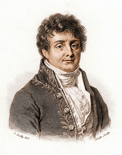
In 1807, the French mathematician Joseph Fourier formulated an insight that reaches far beyond music:
Every periodic signal – no matter how complex – can be written as a sum of sine waves.
The coefficients \(a_1, a_2, a_3, \ldots\) are like the sliders of an equalizer. They tell you how much of each frequency is contained in the signal. Two descriptions of the same thing – like two languages for the same thought.
Try it yourself
The visualization is your mixing console. Seven sliders, one for each overtone. Start with the preset "Fundamental" – a pure oscillation. Then choose "≈ Square" and watch how a rectangular wave emerges from just a few sine waves. Then press ▶ Play and look to the right: there the arrows are spinning. Each overtone is an arrow with its own speed. The sum – the yellow dot – traces the signal.
Spinning Arrows – Again
Since Chapter 1 we have been working with arrows that spin. For three chapters we have added them and watched whether they reinforce or cancel. And now they appear again – right in the middle of music theory. That is no coincidence. It is the same mathematics.
A sine wave is nothing other than a spinning arrow viewed from the side. Imagine a point moving steadily around a circle. Look at the circle from the side – that is, project the point onto the vertical axis. What do you see? The point goes up, comes down, goes up, comes down. A sine wave. Length of the arrow → amplitude of the oscillation. Rotation speed → frequency. Starting angle → phase. Everything that describes a sine wave is contained in a single spinning arrow.
And if a signal is a sum of sine waves, then it is a sum of spinning arrows – laid tip to tail, exactly as at the double slit in Chapter 1. Ptolemy described planetary orbits in the 2nd century with circles upon circles. Fourier decomposed signals in 1807 with the same mathematics. And since Chapter 1 we have been computing quantum amplitudes in exactly this way. Three millennia, three contexts, one structure. Fourier decomposition is arrow addition, sorted by rotation speed.
What This Means for Quantum Mechanics
Quantum systems have eigenfrequencies – discrete values determined by the system. Each eigenfrequency corresponds to a particular energy \(E_n\). And the connection between the two is strikingly direct.
Remember Chapter 3: the action \(S\) determines the arrow angle via \(S/\hbar\). An eigenstate has a fixed energy \(E_n\) – its spatial shape does not change; the only thing that happens is that the arrow rotates. What angle does it accumulate in time \(T\)? The action is simply \(S = E_n \cdot T\), so the angle is \(E_n \cdot T / \hbar\). The rotation speed – the angle per unit time – is therefore:
That is the eigenfrequency. Not a new postulate – it follows directly from "action determines the arrow angle," applied to a state with fixed energy. Each energy state behaves like a pure overtone: an arrow spinning at constant speed. In music: a pure tone. In quantum mechanics: an eigenstate.
How fast do these arrows spin? For an electron in a 1-nanometer box: the slowest arrow (\(n = 1\), energy 0.38 eV) completes about one rotation every 11 femtoseconds. The third fastest (\(n = 3\), energy 3.39 eV) manages nearly one full rotation per femtosecond – nine times faster, because the energies grow like \(n^2\). A femtosecond is a millionth of a billionth of a second. In this world the arrows spin unimaginably fast.
From Signal to Propagator
Now comes the transfer – and it is strikingly direct. Three steps:
Step 1: The propagator \(K(B,A,t)\) is a function of time. If we hold the start and end points fixed and vary only the time, the propagator is a signal – just as the sound of a guitar is a signal.
Step 2: Fourier says: every signal can be decomposed into pure frequencies. So the propagator, too, can be decomposed into pure frequencies.
Step 3: The allowed pure frequencies of a quantum system are exactly the eigenfrequencies \(\omega_n = E_n/\hbar\) – because frequencies that do not correspond to an eigenstate cancel out (like wavelengths that do not fit on a guitar string, as we will see in Chapter 4b). What remains are the eigenstates.
Remember the equalizer: each slider was an overtone. Now replace "overtone" with "energy level." The "volume" of each overtone – how loudly it resonates in the signal – depends on how strongly the eigenstate "lives" at the start and end points. This leads to the formula:
Read that slowly. Every symbol has a meaning you already know:
\(\sum_n\) – sum over all eigenstates (all "overtones" of the system).
\(\phi_n(B)\) – the spatial shape of the \(n\)-th eigenstate, evaluated at the destination \(B\). Think of the guitar string: \(\phi_1\) is one big arc, \(\phi_2\) has two arcs with a node in the middle, \(\phi_3\) has three arcs. Where \(\phi_n(B)\) is large, the eigenstate "lives" strongly at point \(B\). Where \(\phi_n(B)\) is zero, \(B\) is a node – the eigenstate contributes nothing there.
\(\phi_n^*(A)\) – the same shape, evaluated at the starting point \(A\), but with a mirrored arrow (the asterisk). The mirroring appears because the particle departs from \(A\) – and "departing" is the counterpart of "arriving." The counterpart of an arrow is its mirror image across the horizontal axis.
\(e^{-iE_n t/\hbar}\) – an arrow of length 1 that rotates at frequency \(E_n/\hbar\). Just like the overtones in the Fourier visualization above. The minus sign in the exponent determines the rotation direction – a convention that ensures the arrows rotate clockwise, as in Feynman's stopwatch picture.
The same quantity \(K(B,A)\) – once as a sum over paths (Chapter 3), once as a sum over eigenstates (here). Two descriptions of the same physics. Like the equalizer showing the same signal, just in a different representation.
But one crucial question remains open. The Fourier decomposition shows us that there are eigenfrequencies. But where do they come from? What determines the allowed frequencies of a quantum system? Why does hydrogen glow red and not blue? Why do atoms have discrete energy levels instead of a continuum? The answer has to do with standing waves, with boundary conditions – and it is surprisingly simple.
Chapter 4b
The Notes a Quantum System Likes to Play
At the end of Chapter 4a, a question remained: where do the eigenfrequencies come from – the preferred vibrations of a system? Here is the answer.
The Picky String
A guitar string is fixed at both ends. Every vibration must equal zero at both ends. Imagine trying to place a wave on the string whose wavelength does not fit. You push the string into a pattern that is zero at the left end but not zero at the right end – the wave "ends" somewhere in the middle of a peak or trough. That won't work. The string is pinned there. This wave cannot exist on this string.
Which waves do fit, then? Precisely those where an integer number of half-wavelengths fits between the fixed points. Nothing in between. Not 1.5 half-wavelengths. Not 2.7. Only whole numbers.
These are called standing waves – wave patterns that do not travel but vibrate in place. The fixed points force the selection. This selection mechanism is called a boundary condition. Imagine a rope stretched between two door handles. If you shake at the right frequency, a stable pattern builds up – the standing wave. At the wrong frequency, chaotic reflections arise that cancel each other. The system filters itself – only the matching frequencies survive.
Try it yourself
The slider lets you sweep \(n\) continuously from 0.3 to 7.5. At integer \(n\) the wave turns green – it satisfies the boundary condition. At every other value it turns red: at the right edge it reads "≠ 0." Press ▶ Vibration to watch the standing wave oscillate. Switch to ⚛ Quantum particle and note the energy ladder on the right: the spacings keep growing.
From the String to the Atom
Louis de Broglie proposed in 1924: not only light is a wave – so is matter. A particle with momentum \(p\) has a wavelength \(\lambda = h/p\). If you trap a particle in a box – between two impenetrable walls – its wave must fit inside the box. Exactly like the guitar string.
The calculation is three lines long – and the result is surprisingly elegant. The \(n\)-th mode has wavelength \(\lambda_n = 2L/n\) (because exactly \(n\) half-wavelengths must fit inside). The momentum is therefore \(p_n = h/\lambda_n = nh/(2L)\). And the kinetic energy:
We have not introduced any postulate saying "energy must be discrete." All we said was: the particle is a wave, and the wave must fit inside the box. Discreteness arises on its own. It is not put in – it comes out.


From the Box to the Hydrogen Atom
The "particle in a box" is the simplest quantum system. But the principle reaches much further. An electron in a hydrogen atom is not trapped between two walls but caught in the electric attraction of the proton. The potential has a different shape – it goes as \(-1/r\), getting ever deeper the closer the electron comes to the nucleus. But the logic is identical: the electron's wave must "fit." It must fall to zero far from the nucleus rather than grow to infinity. And this boundary condition again selects a discrete spectrum:
The minus sign says: the electron is bound. The factor \(1/n^2\) comes from the shape of the Coulomb potential – different from the \(n^2\) of the box, but arising from the same principle.
When an electron falls from level \(n = 3\) to \(n = 2\), it releases the energy difference as light. For this transition, the result is red light with a wavelength of 656 nanometers – the famous H-alpha line that astronomers see in the spectra of distant galaxies. For \(4 \to 2\) you get turquoise light, for \(5 \to 2\) violet. These are the Balmer lines, which Johann Balmer catalogued empirically in 1885 – thirty years before anyone knew why they exist.
Now you know why. The electron is a wave. The wave must fit inside the atom. Only certain patterns fit. Each pattern has an energy. Transitions between patterns produce light at discrete frequencies. That is the entire secret of spectral lines.
The Zeros That Shouldn't Be
For \(n = 2\), the probability density has a node right in the middle. The particle can be on the left or on the right – but it is never in the middle. How does it get from one side to the other?
The question assumes the particle is a little ball. But it isn't. It is the wave. The whole wave, simultaneously. Only when you measure do you find it at a specific location. Between measurements, the question "Where is it?" has no sharp answer.
And one more thing: the oscillation of an eigenstate is merely a phase rotation – the arrow spins, but its length stays the same. And \(|\psi|^2\) depends only on the length, not the angle. That is why the probability distribution of an eigenstate does not change over time, even though the wave function oscillates. Eigenstates are stationary: their observable properties do not change.
The Word "Quantum"
Max Planck introduced the term in 1900 when he discovered that light energy is exchanged only in packets of size \(E = h\nu\). Twenty-five years later, wave mechanics explained why energy comes in packets. Not because nature mandates it, but because waves living in bounded spaces can only take on certain patterns. A guitar string cannot play just any frequency because it is fixed at both ends. An atom cannot have just any energy because the electron is trapped in the potential of the nucleus. The mechanism is the same.
Chapter 4c
Three Languages, One Physics
The Main Character: \(K(B, A)\)
Everything revolves around a single quantity: the propagator \(K(B,A)\). It answers the most fundamental question of quantum mechanics: how large is the amplitude for a particle to get from point A to point B? There are three entirely different ways to compute this arrow – and all three yield exactly the same result.
Language 1: The Path Integral
Feynman's perspective. Integrate over all possible paths from A to B. Each path contributes an arrow whose angle is determined by the action:
The \(\int \mathcal{D}[x(t)]\) is the path integral – a sum over all conceivable curves \(x(t)\). No eigenstates, no energy levels. Just paths and their actions. Structure emerges only in the summation.
Language 2: The Eigenstate Decomposition
The perspective of wave mechanics. Decompose the propagator into stable patterns – the "pure tones" of the system. Each eigenstate \(n\) oscillates at its eigenfrequency \(E_n/\hbar\):
No paths. Instead, a spectrum – a ladder of energy levels. Each level contributes a spinning arrow, just like the overtones in the equalizer from Chapter 4a. All of chemistry becomes clearest in this language.
Language 3: The Fourier Transform
The mathematician's perspective. The propagator is a function of time. Every time-dependent function can be written as an integral over frequency components:
The frequency spectrum \(\tilde{K}(\omega)\) has peaks at the eigenfrequencies \(\omega_n = E_n/\hbar\). In between, it is zero. The Fourier transform finds the eigenstates without you having to know them beforehand.
Do You See It?
Look at the three formulas again. They look different – but they share the same architecture:
Path integral: \(K = \displaystyle\int \mathcal{D}[x]\; e^{\,i\,S[x]\,/\,\hbar}\) — integrate over paths, weighted by \(e^{i \cdot \text{action}}\)
Eigenstates: \(K = \displaystyle\sum_n \underbrace{\psi_n(B)\,\psi_n^*(A)}_{\text{Fourier coeff.}}\; e^{-i\,E_n\,t\,/\,\hbar}\) — sum over modes, weighted by \(e^{i \cdot \text{energy} \times \text{time}}\)
Fourier: \(K = \displaystyle\int \tilde{K}(\omega)\; e^{-i\,\omega\,t}\;d\omega\) — integrate over frequencies, weighted by \(e^{i \cdot \text{frequency} \times \text{time}}\)
Three times the same pattern: integrate (or sum) over all possibilities, and give each possibility a spinning arrow \(e^{i \cdot \text{something}}\). In the path integral, that "something" is the action of a path. For the eigenstates, it is energy times time. For Fourier, it is frequency times time. The structure is identical. Only the variable being summed over differs: paths, energy levels, or frequencies.
This is the deep insight – and it is no coincidence. It follows from the fact that quantum mechanics is linear: every solution can be written as a superposition of other solutions. This property forces the existence of different "bases" (paths, eigenstates, frequencies) between which you can freely switch – like different coordinate systems for the same space.

The Triangle
The three languages form a triangle. Each side connects two perspectives:
Paths ↔ Eigenstates: you can regroup the sum over paths so that it becomes the sum over eigenstates. Like a book that exists in both English and French: different sound, same content.
Eigenstates ↔ Fourier: the eigenstate decomposition is the Fourier decomposition applied to the signal "propagator." Mathematically it is literally the same thing.
Fourier ↔ Paths: both are "sums over everything" – only the "everything" differs: time points vs. frequencies, paths vs. amplitudes.
Why Three Languages?
Each makes something visible that the others hide. The path language makes interference tangible – you see why the classical path dominates and why quantum effects vanish for large objects. But try using the path integral to compute the energy levels of hydrogen – it's a nightmare.
The eigenstate language makes spectra tangible – the energy ladder, the allowed transitions, all of chemistry. But try using it to explain why a ball flies in a parabola – it's cumbersome.
The Fourier language is the bridge. It shows that eigenstates are nothing but frequency components of a signal. It connects quantum mechanics with signal processing, acoustics, and optics. Its weakness: it is abstract. It says "there are peaks in the spectrum," but it tells no physical story about why.
The strength of one language is the weakness of another. Together they form a complete picture. Physicists switch between them constantly – sometimes in the middle of a calculation – like a bilingual person who starts a sentence in English and finishes it in French because the better word happens to be in the other language.
The Equivalence – Not Obvious, but Provable
That the three languages say the same thing is not a metaphor. It is a mathematical theorem. Heisenberg arrived in 1925 via matrices, Schrödinger in 1926 via wave equations, Feynman in 1948 via path integrals. Each initially thought he had discovered something new. Then it turned out: it was the same thing three times over. Nature had a single structure, and three physicists had found it from three different directions – like three tunnels that meet in the same chamber.
What you now know: In Chapter 1 you added arrows. In Chapter 2 you learned the two rules. In Chapter 3 you understood the path integral and stationary phase. In 4a you met the Fourier decomposition. In 4b you saw where eigenstates come from. And now you know: all three perspectives say the same thing. That is, in broad strokes, the formalism of non-relativistic quantum mechanics. Professors need a semester for this. The calculation technique is missing – but the way of thinking is there.
Why does quantum mechanics have this structure? One possible answer: because it is linear. The Schrödinger equation is linear – if \(\psi_1\) and \(\psi_2\) are solutions, then so is \(\psi_1 + \psi_2\). Linearity is precisely the property that makes Fourier decompositions possible. And linearity is also the property that guarantees the superposition principle – that quantum states can be superposed. The equivalence of the three languages and the superposition of quantum mechanics are the same fact, viewed from two angles.
Perhaps the deepest lesson of quantum mechanics: not that cats are simultaneously alive and dead. But that nature is richer than any single description we can give of it.
Chapter 4d
From Particles to Fields – and Why You Can Never Quite Pin Down a Particle
The Universe’s Equalizer
In Chapter 4a you decomposed a signal in time into frequencies – like an equalizer that splits a song into bass, mids, and treble. Now we do the same thing, but with a field in space.
Imagine a field that fills all of space – like a temperature distribution, except instead of temperature it carries a physical quantity at every point. The Fourier decomposition breaks this field into modes: sine waves of various wavelengths. The same trick as the equalizer – only instead of a slider per frequency, now a slider per wavelength.
Mathematically it looks almost identical to 4a:
The same \(e^{i \cdot \text{something}}\) as everywhere in this blog. Only now \(x\) is a position rather than a time, and \(k\) is a wavenumber rather than a frequency.
Every Slider Is a Swing
Here comes the conceptual leap. Each individual Fourier mode of this field – each sine wave with a particular wavelength – behaves mathematically like a harmonic oscillator. A child on a swing. It has an amplitude and a frequency.
In Chapter 4b you saw: a particle in a box has discrete energy levels. The harmonic oscillator has discrete levels too, but they are evenly spaced:
The \(n\) counts excitation levels: \(n = 0\) (ground state), \(n = 1\) (first excitation), \(n = 2\) (second), and so on. Now the punchline:
“Quantizing a field” means: giving each Fourier mode discrete energy levels. And the excitation number \(n\) of a mode means: “There are \(n\) particles with this wavelength.”
The analogy: imagine an organ with infinitely many pipes, one per wavelength. Each pipe can be silent (\(n = 0\), vacuum), hum softly (\(n = 1\), one particle), louder (\(n = 2\), two particles). “Creating a particle” means turning a pipe up by one notch.
Why Particles Can Be Created and Destroyed
In Chapters 1 through 4c, the world was like this: there is a particle, and it has a wave function. The particle was given – you could ask where it is or how fast it moves, but not whether it exists.
In quantum field theory (QFT), things are different. Here the field is fundamental, not the particle. A “particle” is not an independent entity – it is an excitation of a mode. That is why particles can be created and destroyed: you are not conjuring matter from nothing, you are turning a slider up or down.
(The full story involves special relativity, but it does not change the Fourier structure – it adds an elegant frame around it.)
Why You Can Never Pin Down a Particle
Now we reach the heart of the matter – and here the circle back to Chapter 4a closes.
A single Fourier mode \(e^{ikx}\) is a sine wave stretching across all of space. It has a perfectly defined momentum (via de Broglie: \(p = \hbar k\)). But where is the particle? Nowhere and everywhere – the wave has no preferred position.
Remember the equalizer from 4a? A pure tone has no beginning and no end. A sharp “click” needs all frequencies. The exact same thing holds in space: a pure momentum wave has no location. A localized particle needs all wavelengths.
To build a “particle-like” thing – something that is roughly here and not there – you must superimpose many Fourier modes. The result is a wave packet: a localized bump in space.
But the more modes you superimpose, the wider the momentum distribution becomes. And conversely: the fewer modes, the sharper the momentum – but the more smeared out the particle is in space. There is no escape.
Try it yourself – drag the slider and watch position and momentum fight each other:
This is the famous Heisenberg uncertainty relation:
And here is the crucial point: this is not a separate postulate. It is not a law of nature that someone discovered. It is a mathematical theorem about Fourier transforms. It holds equally in signal processing, in acoustics, in radio engineering. In communications engineering it is called the bandwidth theorem: sending a sharp pulse requires a wide bandwidth. Heisenberg is the same mathematics, applied to matter waves.
Summary: The Fourier modes from 4a, the discrete levels from 4b, the three languages from 4c all lead to one conclusion: particles are not points. They are excitations of modes. And modes cannot be simultaneously perfectly localized and perfectly monochromatic. That is the uncertainty relation.
In the bonus chapter we see another consequence: what happens when two particles share a set of arrows – entanglement.
Bonus Chapter
Entanglement – When Two Particles Share a Secret
Two Photons, One Pair of Arrows
An atom emits two photons simultaneously – one to the left toward Alice, one to the right toward Bob. Nature has entangled these two photons. That means: there is not one arrow for photon A and a separate arrow for photon B. There is a joint set of arrows for the pair.
There is an arrow for "Alice measures ↑ AND Bob measures →."
And an arrow for "Alice measures → AND Bob measures ↑."
No arrow points to "both ↑" or "both →." Therefore: if Alice measures ↑, Bob must measure →.
"That's Trivial!"
You might think: the photons fixed their polarization at the moment of creation – like a pair of gloves, one sent to Berlin and the other to Tokyo. Open the Berlin suitcase and find the left glove, and you instantly know the right one is in Tokyo. No magic.
Einstein thought exactly that. He called quantum mechanics "incomplete" and suspected hidden variables.
Bell's Stroke of Genius
In 1964, the Northern Irish physicist John Bell had an idea that changed everything. He asked: if the photons really did have their properties in advance – like the gloves – what maximum correlation could you expect between Alice's and Bob's measurements?
The Limit of the Gloves – with Numbers
Bell proposed the following experiment. Alice randomly chooses one of two measurement directions for each photon: \(a_1 = 0°\) or \(a_2 = 45°\). Bob likewise: \(b_1 = 22{,}5°\) or \(b_2 = 67{,}5°\). Each measurement yields +1 or −1. After thousands of runs they compute the correlation \(E(a, b)\) – how often they agree minus how often they disagree – for each of the four angle combinations.
Now the decisive quantity. Define:
If hidden variables exist – if every photon has fixed its answers for all possible angles at birth – then you can show in three lines that \(|S| \leq 2\). The proof: each individual photon pair carries predetermined outcomes \(A_1, A_2, B_1, B_2 = \pm 1\). Substitute: \(S_{\text{single}} = A_1(B_1 - B_2) + A_2(B_1 + B_2)\). Since \(B_1\) and \(B_2\) are each \(\pm 1\), either \(B_1 - B_2 = 0\) or \(B_1 + B_2 = 0\) – one of the two terms always vanishes. So \(|S_{\text{single}}| = 2\). Averaged over many pairs: \(|S| \leq 2\).
This is the CHSH inequality – the experimentally testable version of Bell's limit. No matter how cleverly the "gloves" are programmed: \(S\) can never exceed 2.
What Quantum Mechanics Predicts
The arrow rules say: at an angle difference \(\theta\) between Alice and Bob, the outcomes agree with probability \(\cos^2(\theta)\). The correlation is \(E(a, b) = \cos(2(a - b))\). Plugging in Bell's optimal angles:
| Pair | Angle difference | Correlation |
|---|---|---|
| \(E(0°,\; 22{,}5°)\) | 22.5° | +0.707 |
| \(E(0°,\; 67{,}5°)\) | 67.5° | −0.707 |
| \(E(45°,\; 22{,}5°)\) | 22.5° | +0.707 |
| \(E(45°,\; 67{,}5°)\) | 22.5° | +0.707 |
The trick: three of the four pairs have 22.5° difference (strong correlation: +0.707). The fourth has 67.5° (anti-correlation: −0.707). But the minus sign in the \(S\) formula flips this anti-correlation. All four terms add up:
2.83 > 2.
Stop. Wait. This is the moment. The gloves allow at most 2. Quantum mechanics says 2.83. This is not a small difference, not a rounding error, not a matter of interpretation. It is a mathematical theorem: no theory with predetermined properties can reach \(S = 2{,}83\). Nature does it anyway.
What the Experiment Says

Alice and Bob set their detectors to different angles. For each photon pair, both record their result: +1 or −1.
At equal angles: perfect anti-correlation. Always.
At 90° difference: no correlation. Completely random.
In between: a smooth cosine curve – and this curve lies beyond Bell's limit.
And the experiments? Aspect (1982): \(S = 2{,}70\). Weihs and Zeilinger (1998): \(S = 2{,}73\). Hensen in Delft (2015, the first loophole-free test): \(S = 2{,}42\). All above 2. All consistent with \(2\sqrt{2}\). In 2022, Alain Aspect, John Clauser, and Anton Zeilinger received the Nobel Prize for this work.
What Entanglement Is – and What It Isn't
Entanglement is not communication (Bob cannot read anything from his results alone), not teleportation (nothing travels faster than light), and not mysticism (it is mathematics, confirmed in the lab).
What entanglement is: the arrows belong to the pair, not to the individual particles. Nature's bookkeeping can be nonlocal – not because information travels faster than light, but because the bookkeeping encompassed the whole system from the start.
Try it yourself
In the visualization you can run Bell's experiment yourself. Choose measurement angles for Alice and Bob. Press "Measure" and observe the results. Save data points at various angle differences and watch the correlation curve break through Bell's limit. The gloves could not have done that.
Epilogue
What Happens When You Look?
So far we have described a quantum system evolving undisturbed – with nobody looking. The wave function oscillates, the arrows spin, the eigenstates superpose. Everything is smooth and deterministic.
But what happens when you measure? When you catch an electron that exists in a superposition of "here" and "there" with a detector – and suddenly it is here, only here, with certainty?
Where did the superposition go? Was the electron already "here" before, and we just didn't know? Or did the measurement create reality? And if so – what exactly counts as a "measurement"?
That is the famous measurement problem – the open wound of quantum mechanics. For nearly a hundred years the sharpest minds in physics have been arguing about it, and there is no consensus.
We will talk about that – soon.
Frequently Asked Questions
What is the path integral?
The path integral is a formulation of quantum mechanics developed by Richard Feynman in 1948. Instead of solving a wave equation, you sum over all possible paths a particle can take from A to B. Each path gets an 'arrow' (a complex amplitude), and the sum of all arrows gives the total probability.
Why does the interference pattern disappear when you measure?
When you measure which slit the particle goes through, the two paths become distinguishable. You only add arrows when paths are indistinguishable. Make them distinguishable, and there is only one arrow per run – no addition, no interference. It is not mysticism, it is bookkeeping.
What is the difference between diffraction and interference?
Physically, there is no sharp difference – Feynman himself said nobody has ever satisfactorily defined the distinction. Diffraction is the spreading behind a single slit, interference is the superposition from two or more slits. Both are the same principle: adding arrows.
Why is the exponential function the only possible quantum amplitude?
The quantum rules require: actions add for sequential path segments, amplitudes multiply. The only continuous function that turns addition into multiplication is the exponential function. Combined with the requirement of equal arrow length (|A|=1), only e^{iS/ħ} remains.
Why are Fourier modes used in quantum field theory?
In QFT, a field in space is decomposed into Fourier modes – sine waves of various wavelengths. Each mode behaves like a harmonic oscillator with discrete energy levels. The excitation number of a mode corresponds to the number of particles with that wavelength. Fourier modes are therefore not a mathematical convenience but the fundamental objects of the theory.
Is the uncertainty principle a physical law?
No – it is a mathematical theorem about Fourier transforms. If a function is narrow in position space (localized), its Fourier transform must be wide (many wavelengths), and vice versa. In physics this translates to: position and momentum cannot both be arbitrarily sharp at the same time. The same principle holds in signal processing as the bandwidth theorem.
Read next
Related posts on ki-mathias.de:
- What Quantum Computers Do — Qubit, Bloch sphere, Qiskit
- Eigenvalues & AI — Kernels, PageRank, Neumann series