Deepfakes Explained

Q: What is the difference between PCA and an autoencoder?

PCA is a linear dimensionality reduction. An autoencoder is the nonlinear generalization and can learn arbitrarily complex manifolds.

Q: Why can we still sometimes detect deepfakes?

Models trained on insufficient data leave artifacts: unnatural blinking, inconsistent lighting, patterns in the frequency spectrum.

From vectors and autoencoders to the face swap – the math behind the illusion

1The Motivation

In summer 2024, I gave a tech talk at my company. The topic: nonlinear operations in high-dimensional spaces. Sounds abstract. It is – until you realize this is exactly the math behind deepfakes.

The question I wanted to answer: How does a computer transfer one person's face onto another so convincingly? The answer goes through vectors, matrices, dimensionality reduction, the kernel trick, and neural networks – and in the end, it's shockingly simple.

This post follows the arc of my presentation. Each chapter builds on the previous. By the end, you'll understand why a swapped decoder is enough to fake a face.

2Vectors & Matrices

Let's start at the beginning. A vector is a list of numbers. Two numbers describe a point in the plane, three a point in space:

$$\vec{A} = \begin{pmatrix} 2 \\ 3 \end{pmatrix} \quad \text{(2D)} \qquad \vec{B} = \begin{pmatrix} 1 \\ 4 \\ 2 \end{pmatrix} \quad \text{(3D)}$$

A matrix is a table of numbers that turns one vector into another. A 3×3 matrix can rotate, scale, or project a vector – all with a single multiplication:

$$\vec{v}_{\text{new}} = R \cdot \vec{v}_{\text{old}}$$

Try it – transform a vector live below:

3Orthogonality

A vector in 3D space can be written as a combination of three basis vectors $\vec{i}$, $\vec{j}$, and $\vec{k}$. These are perpendicular to each other – orthogonal. Each describes a completely independent direction.

What does that mean for real data? Take human attributes:

Shoe size ↔ height: related (correlated)
Age ↔ weight: partially related
Eye color ↔ income: completely independent (orthogonal)

Orthogonal features carry no redundant information. And that's what becomes important later: if we can find and remove redundancy in data, we need fewer dimensions.

4Blind Source Separation

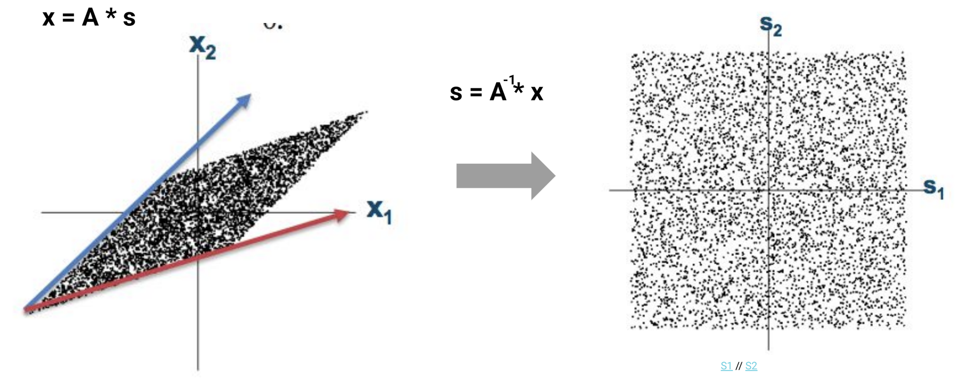
An example of orthogonality's power: the cocktail party problem. Someone speaks while music plays. Two microphones record the mixture. Mathematically:

$$\mathbf{x} = A \cdot \mathbf{s}$$

where $\mathbf{s}$ are the source signals and $A$ is the mixing matrix. If we can invert $A$:

$$\mathbf{s} = A^{-1} \cdot \mathbf{x}$$

The correlated, mixed data (a slanted parallelogram) becomes decorrelated, separated signals (a clean square). The signals are now orthogonal to each other.

Blind Source Separation: Inverting the mixing matrix — Left: correlated mixed signals. Right: separated source signals after decorrelation.

5High-Dimensional Data

So far we've thought in 2 or 3 dimensions. But mathematically, you can construct any number. A tesseract is a cube in 4D space – you can barely visualize it, but you can compute with it just fine:

What does this have to do with images? A black-and-white image with 10×20 pixels has 200 pixel values. You can think of it as a 200-dimensional vector – each pixel is a coordinate.

Are these 200 dimensions orthogonal? No. Neighboring pixels are highly correlated. If one pixel is bright, its neighbor probably is too. There's redundancy in the data.

6Dimensionality Reduction – PCA

Principal Component Analysis (PCA) finds a new coordinate system whose axes are orthogonal and maximize explained variance. The first principal component points in the direction of greatest spread, the second perpendicular to it.

Try it – draw points and watch the PCA axes update live:

The result for images: 10,000 pixels become 2,500 principal components – and the image looks almost identical. The rest was redundancy. That's dimensionality reduction.

For more depth: the Eigenvalues post explains why PCA is mathematically an eigenvalue decomposition of the covariance matrix – and the Fourier post shows why the DCT (which JPEG uses) does essentially the same thing. The post The Eigenprinciple shows that the same eigen-structure also sits behind vibration, search and probability.

7The Limits of Linearity

Dimensionality reduction alone isn't enough. If we linearly interpolate between two faces, this happens:

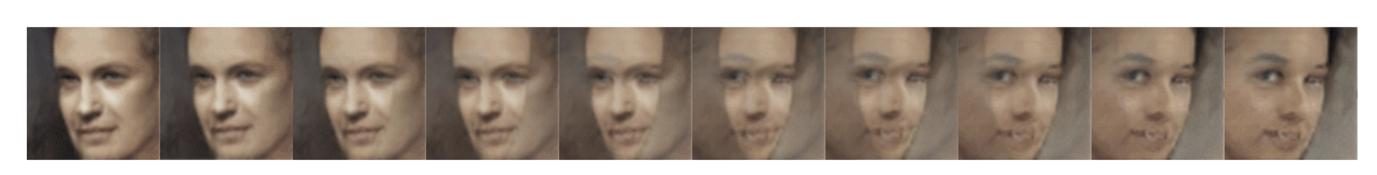
Linear interpolation between faces — Linear interpolation: the intermediate frames are ghosts, not faces.

The intermediate images aren't faces – they're overlays. In pixel space, the straight path between two faces is not a face.

It's completely different with nonlinear interpolation: here, the intermediate frames are actually new, plausible faces.

8The Kernel Trick

And here comes the crucial trick: dimension increase. Data that isn't linearly separable in 2D becomes separable in a higher-dimensional space:

Left: two classes in concentric rings – no straight line can separate them. Right: through the transformation $z = x^2 + y^2$ (lifting into the third dimension), a simple plane becomes the separator.

Together, an elegant double-play emerges:

Dimensionality reduction – to remove redundancy (PCA, DCT)
Dimension increase – to make nonlinearity tractable (kernel trick)

A neural network can do both at once.

9Neural Networks

A single neuron takes multiple inputs $x_i$, multiplies each by a weight $w_i$, sums them up, and passes the result through an activation function $\varphi$:

$$y = \varphi\left(\sum_i w_i \cdot x_i + b\right)$$

The activation function is the key: it's nonlinear. Without it, the entire network would just be one big matrix multiplication – nothing a single matrix couldn't do.

Stack many neurons in layers – input, hidden, output – and you get a neural network. The hidden layers automatically learn which dimensions to expand and which to compress.

For more on emergent properties of such networks: the Emergence post covers exactly this.

10Autoencoders

An autoencoder is a special neural network with an hourglass architecture:

Encoder: compresses a high-dimensional image into a low-dimensional latent space
Decoder: reconstructs the image from the compressed form

The training objective: the output should match the input as closely as possible. The bottleneck in the middle – the latent space – forces the network to keep only the essential information.

That's nonlinear dimensionality reduction. Try it – draw a digit and see how the autoencoder reconstructs it:

11Latent-Space Arithmetic

And now the magic happens. In the latent space, you can do arithmetic on faces like vectors:

$$\text{smiling woman} - \text{neutral woman} + \text{neutral man} = \text{smiling man}$$

This works because the latent space has decomposed faces into orthogonal features: gender, expression, gaze direction, lighting. Every direction in the latent space corresponds to a semantic property.

Explore the latent space of a digit VAE:

If this rings a bell: it's the same trick Word2Vec uses for words. King − Man + Woman = Queen works on exactly the same principle. The Eigenvalues post explains why.

12Deepfakes – The Decoder Swap

And we've arrived. The deepfake trick is shockingly simple:

Train two autoencoders – one for person A, one for person B
Both share the same encoder, but have different decoders
The encoder learns a shared face representation in the latent space
The swap: take an image of person A, run it through the shared encoder – then through the decoder of person B

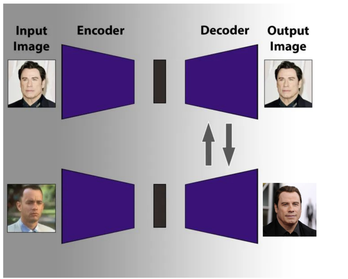
Deepfake encoder-decoder swap — The deepfake trick: encoder of A + decoder of B = appearance of B with expression of A.

The result: the expression and head pose of A, but the appearance of B. A deepfake. Not magic – just dimensionality reduction, dimension increase, and a swapped decoder.

13Ethics & Detection

Deepfakes are unsettling. But understanding beats panic. Knowing how they work helps you spot them:

Artifacts: unnatural transitions at the hairline, ears, teeth
Consistency: lighting on the face doesn't match the rest of the image
Blinking: early deepfakes blink too rarely (training-data bias)
Forensics: frequency analysis reveals GAN-typical patterns in the spectrum

The technology is neutral. It enables medical simulation, film post-production, accessibility (lip-sync for the deaf) just as well. The question isn't whether we should understand it – but whether we can afford not to.

This post is based on a tech talk I gave at P&M Agentur. The original slides and all interactive visualizations are freely available.

Frequently Asked Questions

How does a deepfake work technically?

A deepfake uses two autoencoders with a shared encoder but different decoders. An image of person A is passed through the shared encoder and then reconstructed by the decoder of person B. The result: expression and head pose from A, appearance from B.

What is the difference between PCA and an autoencoder?

PCA is a linear dimensionality reduction – it finds the best orthogonal coordinate system. An autoencoder is the nonlinear generalization: it can learn arbitrarily complex manifolds because its activation functions are nonlinear.

What is the kernel trick?

The kernel trick lifts data into a higher-dimensional space where it becomes linearly separable. Mathematically, you never need the explicit higher dimensions – computing the inner products between data points in the higher space is enough.

Why can we still sometimes detect deepfakes?

Because models trained on insufficient data leave artifacts: unnatural blinking, inconsistent lighting at the hairline or ears, patterns in the frequency spectrum that don't appear in real images.