Fourier, Ocean Waves and 65,536 Frequencies

Chapter 1

Try It Yourself

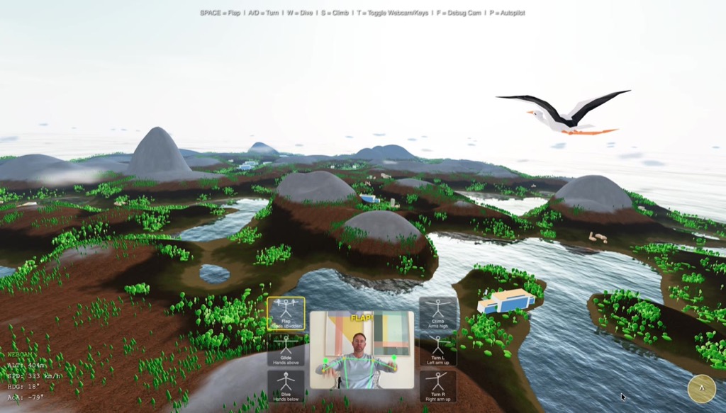
Before we talk — fly first. And watch the water while you do.

Keyboard controls:

SPACE Wing flap   A/D Turn   W Dive   S Climb   T Webcam on/off

When you fly over the sea and see how the waves break differently at each crest, how the horizon is a jagged band rather than a clean line — you are looking at Fourier.

This is the story of a mathematical idea. Joseph Fourier had an insight in 1822 so fundamental that 200 years later it is literally inside every JPEG image, every MP3 file, every AAA ocean shader, and on every modern chip. The idea itself is surprisingly simple. Its consequences are nearly boundless.

We will take it apart. But first, let me explain what you just flew through.

Chapter 2

A World from Nothing — Procedural Landscape

Terrain Without a Single Hand-Placed Vertex

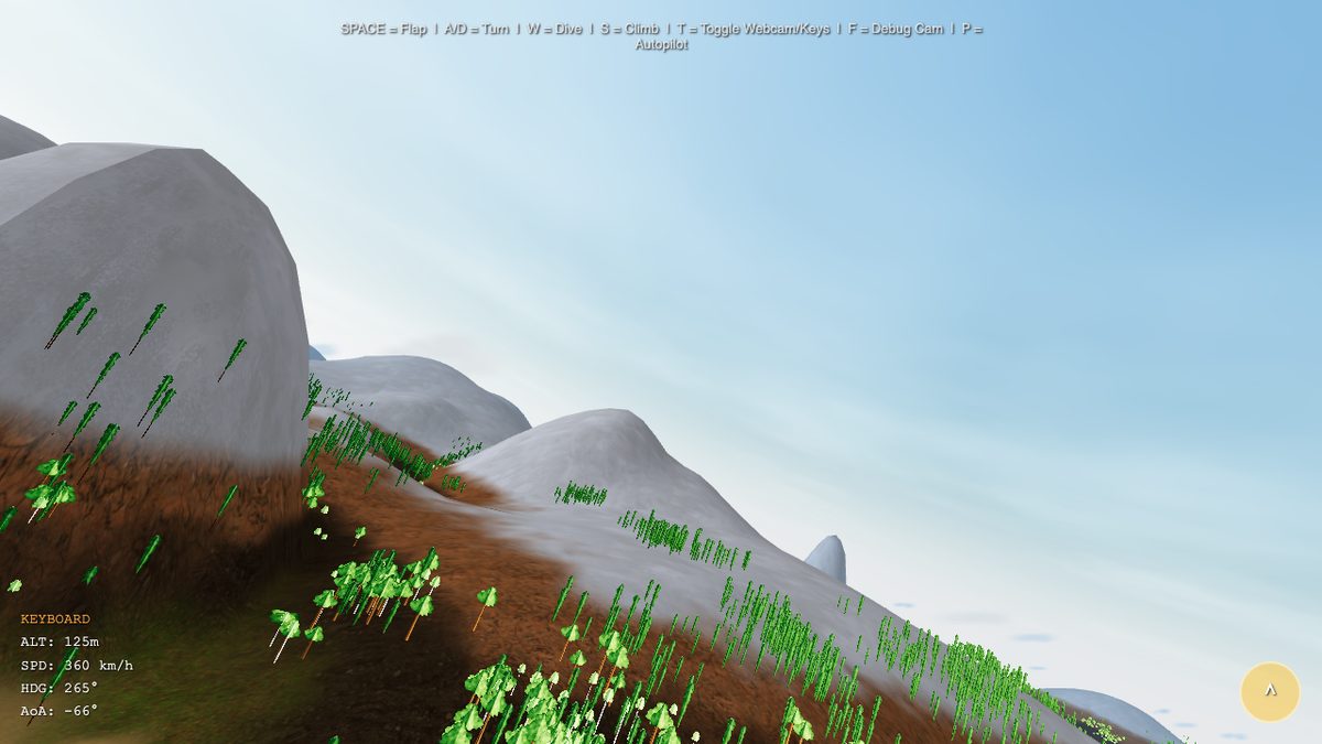
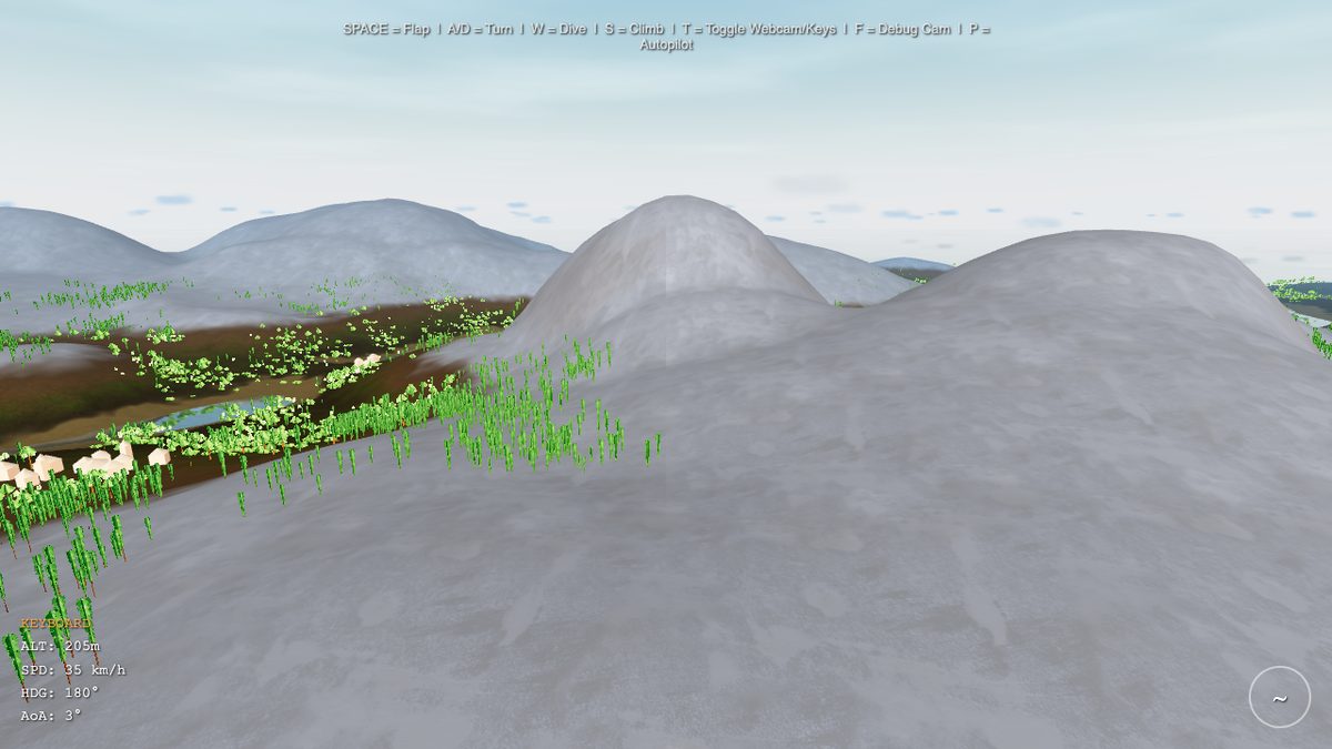
The landscape you flew over was never modeled by a human. No 3D artist placed a hill, no designer drew a valley. Instead, mathematics describes what should appear where, and the computer generates a slightly different but always plausible island on each load.

The core principle is surprisingly simple: Paraboloids as building blocks. Picture a flat table. Now place invisible hills on it — each defined by a center point \((c_x, c_z)\), a radius \(r\), and a height \(h\). At every point on the terrain you add up all contributions:

900 positive paraboloids shape the hills. 270 negative paraboloids carve out valleys. A radial falloff lets the island gently sink into the sea at the edges. The result looks natural because hills in nature actually do arise through the superposition of different processes — tectonics, erosion, deposition. We approximate this process with thousands of simple functions.

Five Texture Layers

Geometry alone creates lumps, not a landscape. Color and texture make the difference. A GLSL fragment shader calculates per pixel which of the five texture layers is dominant: sand at the beach, grass on the hills, earth at mid elevations, rock on steep slopes, snow on the peaks. Transitions run through a smoothstep function that avoids sharp edges.

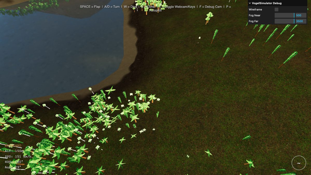
Buildings arise procedurally in a similar way: five types (houses, barns, towers, hotels, high-rises), placed by noise functions in flat coastal areas. A second noise layer separates city from forest zones so that trees do not grow through rooftops. 900 buildings, 100,000 trees — all generated, none placed by hand.

Chapter 3

The Bird Takes Flight — Flight Physics and Webcam

From a Camera with Vertigo to Real Gliding

The terrain was there. But a bird that doesn't fly is just a camera with vertigo. The first approach was a simple arcade model: press a key, go up. It worked technically. But it felt like an elevator with a panorama window — no gliding, no lift, no flying.

So we built an aerodynamic model. The central insight: lift depends on the square of velocity. That is dynamic pressure — the same physics that keeps real birds and aircraft in the air.

The first wing flap did nothing. Gravity won. Every time. The problem: we had forgotten the wing incidence angle. Real bird wings are not flat — they have a built-in angle of attack of about 3° that generates minimal lift even in straight and level flight. Without it, the wing is a board, and a board falls. Six iterations of the physics model later, the balance of gravity, lift and wing flap was right. Until a dive felt dangerous and a loop made the stomach clench.

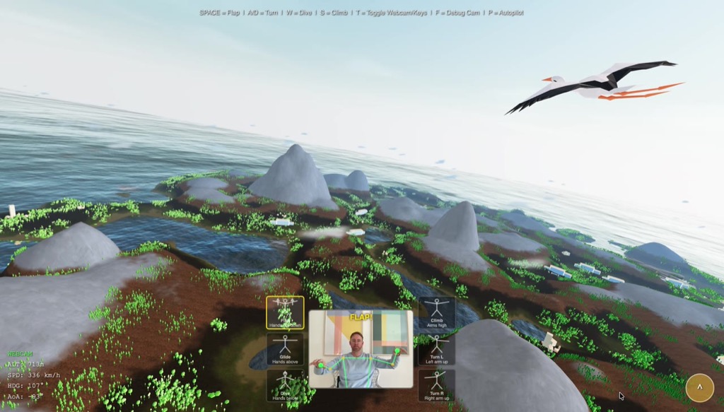
Arms as Wings: MediaPipe Pose Detection

And then the crazy part: what if instead of the keyboard, you use your arms? MediaPipe Pose Detection makes this possible. Google's ML model recognizes 33 body landmarks in real time — directly in the browser, without a server, without the cloud. Shoulders, elbows, wrists: everything we need.

The logic: we measure the height of both wrists relative to the shoulders. Hands high = wings up. Hands low = wings down. The rate of change between them = flap strength. The webcam image is mirrored, landmarks can disappear, detection rate fluctuates with lighting. Our solution was graceful degradation: when MediaPipe detects no pose, the system quietly falls back to keyboard controls. No error, no popup.

The feeling when you first raise your arms and the bird climbs — that is the moment when a technical project becomes something you want to show people.

From webcam game to phone tilt: mobile controls

The webcam controls work beautifully on desktop — but on a phone they are impractical. So for birdybird, the mobile-first offshoot, we built a second control layer: tilt-to-fly. The phone is the stick. Tilt left = bank left. Tilt forward = dive. Shake = flap.

The browser API is called DeviceOrientationEvent and gives three angles: alpha (compass rotation), beta (pitch forward/backward), gamma (side tilt). Sounds simple — in practice we ran into two bigger obstacles.

Problem 1: the axes mean different things to different players. Do you hold the phone flat in front of you like a tray, or upright like a comic book? Portrait or landscape? The raw sensor data differs drastically depending on posture — a hard-coded axis mapping fails for half the users. Solution: a 6-step calibration wizard at first launch. The player holds the phone at rest, left, right, climb, dive, and then shakes it once — we measure the axis deltas for each gesture and determine which sensor axis (beta or gamma) has the widest span for which motion. The result is stored in localStorage; on the next launch the player can choose to reuse the profile or recalibrate.

Problem 2: iOS 13.4+ has a two-permission trap. Since Apple got worried about user tracking via motion sensors, web apps on iOS must request two separate permissions: DeviceOrientationEvent.requestPermission() for the tilt angles, and DeviceMotionEvent.requestPermission() for acceleration (which also drives our shake-to-flap gesture). In our first release we only requested the first one — with the consequence that the calibration step “Flap Wings!” hung forever because devicemotion events never fired. Two-part fix: request both permissions in parallel, plus an 8-second timeout with a “Skip” button for the case where events don't arrive anyway.

Chapter 4

100,000 Trees — Octree and Frustum Culling

The Problem: 60 FPS with 100,000 Objects

An island without forests looks bare. So we placed trees. Many trees. 100,000 trees.

The naive approach: send all 100,000 trees to the GPU every frame and let it draw them. Result: 4 FPS. The computer couldn't keep up. This isn't surprising — even if a tree has only 200 polygons, 100,000 trees are 20 million polygons per frame. A modern GPU can handle that in theory, but the overhead per draw call is the real problem. Each individual draw instruction causes CPU-GPU communication. 100,000 draw calls can bring even the fastest GPU to its knees.

The solution is two-stage: first decide which objects could even be visible. Then draw all visible ones at once. The first step is frustum culling. The second step needs a spatial data structure: the octree.

The View Frustum: Six Planes Define the World

A perspective camera doesn't see a full circle, but a frustum — a truncated cone bounded by six planes:

• Near plane and far plane: minimum and maximum view distance
• Left, right, top, bottom: the four side faces of the view cone

Each of these planes can be written as a normal vector \(\mathbf{n}\) and an offset \(d\). A point \(\mathbf{p}\) lies on the visible side of a plane when:

An object is visible if it lies on the visible side of all six planes — or more precisely: if its AABB (axis-aligned bounding box) at least partially intersects the frustum. The frustum planes are extracted from the camera's projection matrix. Per frame: calculate six plane equations from the current camera position, done.

The naive frustum check has complexity \(O(n)\) — we have to test each of the 100,000 objects against the six planes. At 60 FPS that is 6 million plane tests per second. This is surprisingly fast — CPUs can handle it. But the question is whether we can be smarter: if we know that all trees in a certain region of space lie outside the frustum, we don't need to test the individual trees at all.

The Octree: From \(O(n)\) to \(O(\log n)\)

An octree subdivides space recursively into eight equal-sized cubes. Each cube that contains objects is further subdivided — down to a minimum size or maximum depth. The result is a tree: the root represents the entire world, the leaves are small spatial cells each containing a few objects.

During frustum culling, the algorithm traverses the octree from root to leaves:

1. Check whether the AABB of the current node lies completely outside the frustum. If so: discard the entire subtree. Not a single child is examined.
2. Does the node lie completely inside? Then render all objects in it without further tests.
3. Does it lie partially inside? Recursively check all eight children.

In the ideal case — when a large part of the world is behind the camera — the algorithm discards entire branches of the tree at high levels. Of 100,000 objects, only a few thousand octree nodes are visited at all. The effective complexity approaches \(O(\log n)\) — logarithmic instead of linear.

The octree is built once at load time, in about 80 ms. After that it is static — trees don't move. The query per frame takes under 0.5 ms. This gives us 60 FPS with a world that would naively be unrenderable.

When an InstancedMesh Grows Too Large: Per-Cluster Split

Porting to WebGPU, we hit a second performance wall — this time not because of the number of trees, but because of the structure of our mesh. The forest is rendered from an InstancedMesh: one draw call for all trees, with per-instance position matrices. This is more efficient than 100,000 separate draw calls — but it makes frustum culling impossible, because an InstancedMesh has only one bounding sphere, which must enclose all instances. In our case that sphere was as large as the whole world. Three.js could never discard it, no matter where the camera looked. The vertex shader ran over all ~1 million instances every frame, even when the camera was pointed at an empty quadrant.

The fix: split the monolithic InstancedMesh, after generation, into 20 smaller sub-meshes, one per tree cluster. Each sub-mesh keeps the same material and geometry reference (no memory duplication), but holds only the instance matrices for its own cluster — and therefore a tight bounding sphere. Three.js' frustum culler now works at cluster granularity: trees outside the field of view get thrown out of the pipeline, vertex shader included.

Measured effect in our perf benchmark: ~3× more FPS on WebGPU in every scenario (e.g. 36 → 124 FPS over the ocean, 34 → 71 FPS inside the forest). The classic lesson: bounding-volume granularity is not an implementation detail, it's an architectural decision.

Why This Is Relevant to Fourier

The octree and frustum culling are space partitioning techniques: they solve the problem of which parts of a complex structure are relevant. The Fourier Transform solves the same problem — but in frequency space instead of geometric space. Both ideas are based on the same core intuition: Don't look at everything at once. Understanding comes through decomposition.

Chapter 5

The Fourier Idea

A Claim That Outraged Reasonable Mathematicians

In 1807, Joseph Fourier presented a manuscript to the Paris Académie des Sciences. His claim was simple and simultaneously outrageous: every periodic function can be represented as an infinite sum of sine and cosine functions. Not some functions. All of them. Including square waves with sharp corners. Including sawtooth waves. Including discontinuous step functions that are obviously not smooth.

Lagrange, one of the greatest mathematicians of his time, considered the claim false and blocked publication. Not until 1822 did Fourier's book Théorie analytique de la chaleur appear — and the mathematics of the next two centuries was forever changed.

What is so special about sines and cosines? They are the natural basis functions of periodic phenomena. Everything that vibrates — a guitar string, an ocean wave, the electric field of a laser — vibrates at its core like a sine. The Fourier series says: any arbitrary periodic shape is a mixture of such pure oscillations.

The Fourier Series

Let \(f(t)\) be a periodic function with period \(T\). Then:

The coefficients \(a_n\) and \(b_n\) determine how strongly each frequency \(n/T\) is present in the function. They can be calculated by integration:

What do these integrals mean geometrically? They measure how similar the function \(f\) is to a sine oscillation of frequency \(n/T\). Multiply \(f\) by a cosine and integrate — you get the correlation. Fourier analysis is systematic correlation with all possible frequencies.

The Fourier Transform

For non-periodic functions, the series generalizes to the Fourier Transform:

Here \(\hat{f}(\xi)\) is a complex number for each frequency \(\xi\). The magnitude \(|\hat{f}(\xi)|\) is the amplitude, the argument \(\arg(\hat{f}(\xi))\) is the phase of the respective frequency component. And the inverse — the inverse Fourier Transform — reconstructs the original function:

The Fourier Transform is thus a fully invertible change of coordinates: from the time or spatial domain into the frequency domain and back. No information is lost. It is literally just a different perspective on the same data.

The Analogy to PCA: a Rotated Coordinate System

Anyone who has read the blog post on eigenvalues and AI will recognize a deep parallel. PCA rotates the coordinate system so that the axes align with the directions of greatest variance in the dataset. The new axes are the eigenvectors of the covariance matrix — orthogonal basis vectors that optimally fit the data.

The Fourier Transform does structurally the same thing: it rotates the function-space coordinate system into the basis of sine functions. This basis is orthogonal in the sense of the function inner product — two sine functions of different frequencies are perpendicular to each other:

The difference: PCA finds the optimal basis from the data itself. FFT uses a fixed, universal basis — the frequencies. PCA decomposes into directions of maximum variance; FFT decomposes into oscillation frequencies. Both are orthogonal projections onto a new basis.

Another parallel is found in the cochlea of the human ear: the snail of the inner ear is a mechanical Fourier analysis. Different locations along the basilar membrane resonate at different frequencies — the ear decomposes sound into its Fourier components before the brain processes it. Evolution “discovered” the same mathematics 500 million years before Fourier.

The Fast Fourier Transform: from \(O(N^2)\) to \(O(N \log N)\)

The discrete Fourier Transform (DFT) translates Fourier analysis onto finite sequences of \(N\) samples:

Computed naively: for each of the \(N\) output values \(X[k]\) you must sum over all \(N\) input values. That is \(O(N^2)\). For \(N = 65{,}536\) — the resolution of our ocean simulator — that would be \(4.3 \cdot 10^9\) complex multiplications. Per frame. Impossible.

In 1965, James Cooley and John Tukey published an algorithm that computes the DFT in \(O(N \log N)\): the Fast Fourier Transform (FFT). The idea: the DFT of a sequence of length \(N\) can be split into two DFTs of length \(N/2\) — one for the even, one for the odd indices. This divide-and-conquer scheme is applied recursively until you reach DFTs of length 1 (trivial result). With \(\log_2(N)\) recursion levels and \(N/2\) operations per level:

For \(N = 65{,}536 = 2^{16}\): DFT would need \(4.3 \cdot 10^9\) operations, FFT needs \(5.2 \cdot 10^5\). 8,000 times faster.

The data flow of the Cooley-Tukey algorithm looks like a butterfly when visualized: each stage combines results in pairs via complex rotations around the twiddle factors \(W_N^k = e^{-2\pi ik/N}\). This visual impression gave the procedure its name: the butterfly algorithm.

Chapter 6

Fourier Everywhere — Images, JPEG, MP3, Phase Correlation

Images in Frequency Space

The Fourier Transform is not limited to time-dependent signals. Images are two-dimensional functions — the brightness at each pixel as a function of \((x, y)\). So there is also a 2D FFT:

What do the frequencies mean in images? Low frequencies — points near the center of frequency space — encode slow changes: backgrounds, color gradients, the coarse structure of the image. High frequencies — points at the edges — encode rapid changes: edges, fine textures, details.

This decomposition has an important practical consequence: most natural images have a strongly clustered energy distribution. Almost all information is in the low frequencies. The high frequencies contribute little — and they can therefore be discarded or coarsened without the human eye noticing the difference.

The 2D FFT also enables fast convolution: applying a blur filter to an image is an expensive convolution operation in spatial space (\(O(N^2 \cdot K^2)\) for an \(N\times N\) image with a \(K\times K\) kernel). In frequency space it is a simple pointwise multiplication (\(O(N^2)\)). The typical path is therefore: compute FFT, multiply, inverse FFT — already significantly faster than direct convolution for moderately large images.

JPEG: Fourier in 8×8 Blocks

Every JPEG image you have ever seen is full of Fourier mathematics — in a slightly modified form. JPEG uses the Discrete Cosine Transform (DCT), a close relative of the DFT that produces only real numbers and proved better suited for image compression.

The JPEG compression algorithm works in five steps:

1. Division: The image is split into 8×8-pixel blocks.
2. DCT: Each block is transformed into 64 frequency coefficients — from DC (the average brightness) to the highest spatial frequencies.
3. Quantization: The coefficients are divided by a quantization matrix and rounded. Low frequencies are preserved finely, high frequencies are coarsened. This is the lossy step.
4. Run-length encoding: Coefficients are read in zigzag order — from low to high frequencies. Since high frequencies are often zero after quantization, long runs of zeros arise that are coded compactly.
5. Huffman coding: Lossless compression of the quantized values.

The result: an image saved at quality 80 precisely retains the low frequencies (coarse structure) and coarsely quantizes the high frequencies (fine details). The human eye usually only notices the difference when the quality is set very low and the typical JPEG artifacts — blocky 8×8 patterns — become visible. Those are literally the 8×8 DCT blocks showing through under extreme compression.

MP3 and MDCT: Fourier for the Ear

MP3 does something similar for audio. The Modified Discrete Cosine Transform (MDCT) decomposes the audio signal into frequency bands — similar to the cochlea of the inner ear. A psychoacoustic model then exploits an insight: quiet frequencies sitting next to loud ones are masked by the hearing system and can be discarded without most people noticing the difference. A more detailed discussion of audio perception, the cochlea and the harmonic series can be found in the blog post on the mathematics of music.

Phase Correlation: Automatic Video-Music Synchronization

A lesser-known application: phase correlation for automatically finding matching musical passages. When cutting videos, you sometimes have two similar audio sequences — two takes of the same piece of music — and need to determine precisely at which point one aligns with the other.

In the time domain that would be an expensive cross-correlation: try all possible offsets, compute the correlation for each one. In the frequency domain it is a one-liner: compute FFT, form the quotient of the normalized spectra, inverse FFT — the result is a spike precisely at the offset with maximum alignment. Exact synchronization search in \(O(N \log N)\) instead of \(O(N^2)\).

And with that we arrive at the decisive question: what happens when you apply the Fourier Transform in reverse — when you don't analyze a signal, but synthesize a signal from a frequency spectrum?

Chapter 7

From Statistics to Ocean — iFFT on the GPU

What Happens When You Run Fourier in Reverse?

Fourier analysis takes a signal and finds the frequencies it contains. The inverse Fourier Transform (iFFT) does the opposite: it takes a frequency spectrum and synthesizes a signal from it. You define which frequencies should be present with what amplitude and phase — and the iFFT builds the corresponding waveform.

That is exactly what the ocean simulator does. Not with audio signals, but with water surfaces.

The Phillips Spectrum: Oceans in Frequency Space

Owen Phillips formulated a statistical model in 1957 for how wave energy distributes across different frequencies and directions — depending on wind speed, wind direction, and the so-called fetch (the distance over which the wind has blown). The result: the Phillips spectrum:

Here \(\mathbf{k}\) is the wave vector in frequency space, \(k = |\mathbf{k}|\) its magnitude, \(L = v^2/g\) the characteristic wavelength at wind speed \(v\) and \(g = 9.81\,\text{m/s}^2\), and \(\hat{\mathbf{w}}\) the wind direction. The squared dot product \(|\hat{\mathbf{k}} \cdot \hat{\mathbf{w}}|^2\) suppresses waves perpendicular to the wind.

This spectrum lives entirely in frequency space: every point on a 2D grid corresponds to a wave frequency and direction — not a position on the water. It describes no concrete wave, but a probability distribution of waves.

From Statistics to Wave: Tessendorf's Method

The British mathematician and oceanographer Owen Phillips provided the statistics in 1957. The first FFT-based ocean visualization came in 1987: Gary Mastin, Peter Watterberg and John Mareda published in IEEE Computer Graphics and Applications the paper "Fourier Synthesis of Ocean Scenes" — the first application of the FFT method in computer graphics.

The breakthrough for film and games came in 2001: Jerry Tessendorf of Industrial Light & Magic published his paper "Simulating Ocean Water" for the SIGGRAPH courses — the standard reference to this day. Tessendorf did not invent the method, but he worked it out so clearly and tailored it so well to the needs of film production that his paper became the de facto textbook.

The method in five steps:

1. Initialize spectrum: For each point \((k_x, k_y)\) of a 512×512 frequency grid, compute \(P(\mathbf{k})\) from the Phillips spectrum. Multiply by random Gaussian noise to obtain realistic phase variance.
2. Time evolution: Each frequency propagates with the dispersion relation for deep-water waves: \(\omega(\mathbf{k}) = \sqrt{g\, k}\). Multiply each spectral value by \(e^{i\omega t}\) for the current time \(t\).
3. iFFT on the GPU: Apply the inverse 2D FFT. The result is a 512×512 heightmap — the wave height at each point of the grid.
4. Displacement and normals: A second iFFT pass generates horizontal displacements (for the characteristic sharp wave crests) and a third generates the surface normals for correct light refraction.
5. Rendering: The displacement map displaces the vertices of the water mesh; the normal map controls the reflections.

At 512×512 resolution that is \(512^2 = 262{,}144\) spectral values. Each value represents a single wave frequency and direction. The iFFT combines all 262,144 frequencies into a single, coherent water surface. 65,536 visible waves per frame is a conservative measure of what the simulator's ocean actually represents.

The Butterfly Algorithm on the GPU

On the CPU, even the FFT would be too slow for 60 FPS: a 512×512 2D FFT comprises 512 row-wise 1D FFTs of length 512, then 512 column-wise 1D FFTs — 1,024 FFTs in total at 1,310,720 operations each. On the GPU this becomes a pipeline of fragment shaders:

A 1D FFT of length 512 has \(\log_2(512) = 9\) butterfly stages. Each stage renders into a float framebuffer texture target. The result is used as input for the next stage — ping-pong buffering between two textures. Nine render passes, and the rows are done. The same transposed for the columns. At the end, the displacement map and the normal map are available as textures that are directly fed in as vertex shader uniforms.

The JavaScript implementation chain running in the simulator is the result of a decade of open-source work:

• 2013 — WebGL demo by David Li (david.li/waves/), implementing Tessendorf's mathematics with fragment shaders
• 2014 — Three.js port by Aleksandr Albert
• 2015 — reusable Three.js module by Jérémy Bouny (github.com/jbouny/ocean)
• 2023 — Three.js update by Phil Crowther, published at philcrowther.com/Aviation
• 2023 — GLSL3/WebGL2 shader upgrade by Attila Schroeder

The module Ocean3.js — approximately 570 lines of WebGL2 code — is licensed under CC BY-NC-SA 3.0. The license is explicit: use permitted for non-commercial purposes with attribution. The authors are David Li, Aleksandr Albert, Jérémy Bouny, Phil Crowther and Attila Schroeder; the scientific foundation is Tessendorf (2001) and Mastin et al. (1987), the wave statistics come from Phillips (1957). The simulator acknowledges this entire chain.

The Integration

The actual integration work was mechanical but precise: the Water class from Three.js needed to use the FFT normal map instead of its default texture, and the FFT displacement map had to be injected into the vertex shader via shader string injection:

// WaterPlane.js — hybrid construction
const ocean = new Ocean(renderer, {
  Res: 512, Siz: 2400,   // 512×512 grid, 2.4 km tile size
  WSp: 18, WHd: 295, Chp: 1.5  // Wind 18 m/s, direction 295°, choppiness 1.5
});

const water = new Water(geometry, {
  waterNormals: ocean.normalMapFramebuffer.texture, // FFT normal map
  sunColor: 0xffeedd,
  sunDirection: sunPos.normalize(),
});

// Inject displacement map into vertex shader via string injection
water.material.uniforms.oceanDisplacement = {
  value: ocean.displacementMapFramebuffer.texture
};
water.material.vertexShader =
  'uniform sampler2D oceanDisplacement;\n' +
  water.material.vertexShader
    .replace('void main() {',
      'void main() { vec3 oceanDisp = texture2D(oceanDisplacement, uv).rgb;')
    .replace(/vec4\s*\(\s*position\s*,\s*1\.0\s*\)/g,
      'vec4(position + oceanDisp, 1.0)');

Eleven lines of glue code for an ocean simulation that runs an iFFT pipeline on the GPU in the background. The Water class delivers the sun reflection; the iFFT generates the physically grounded, animated wave surface.

From Ocean3 to Ocean4: The Migration to WebGPU

Everything described so far runs on WebGL2 — the graphics API that reached most browsers in 2017. Meanwhile, WebGPU has arrived: a significantly more modern API that allows direct compute shaders (not just fragment and vertex) and dramatically more efficient pipeline configuration. Chrome and Firefox have supported WebGPU since 2023, Safari since iOS 18.

The WebGPU successor Ocean4.js replaces the fragment-shader pipeline with WGSL compute shaders. Instead of nine render passes with ping-pong buffering per 1D FFT, there are now compute dispatches that write directly into StorageTextures. For us, the migration meant: double the whole renderer path, replace ShaderMaterial with TSL NodeMaterial, swap Ocean3 for Ocean4. For birdybird, WebGPU is now the default; WebGL2 continues as a fallback for older devices.

Cascaded Spectra: Three Wave Spectra Layered

A single FFT tile produces surprisingly uniform waves — across a wide ocean you mostly see one wavelength and its harmonics. Real seas layer far more scales on top of each other: swell of 100+ m, wind chop of 10-30 m, tiny ripples below 1 m. A cascaded architecture solves this (see Threejs-WebGPU-IFFT-Ocean by Attila Schroeder): three parallel FFT spectra with different tile sizes (e.g. 250 m / 17 m / 5 m), whose displacement and normal maps are summed on the wave surface.

A full integration of his system would have been several days of work (quadtree chunks, his own ECS framework, nine WGSL shader files). As an interim step we built a “poor man's cascaded ocean”: three Ocean4 instances run in parallel at different tile sizes (2400 m, 300 m, 40 m), and their outputs are summed in the vertex and fragment shaders. It's available for testing via ?ocean=cascaded — at about 60 % FPS cost, but with a palpably livelier surface: big swell and fine sparkle ripples coexist on the same water.

Chapter 8

How We Built It

A Ticket System as the Foundation

The project started with a blank canvas and a decision: no Unity, no Unreal, but pure JavaScript with Three.js directly in the browser. No app, no store, no download. The user opens a URL and flies.

I was the product owner. The vision, the aesthetic decisions, the "that feels wrong, do it differently" — that came from me. Claude Code was everything else: project manager, developer, tester in one instance.

Claude Code set up a ticket system in Markdown at the start — 40 tickets, divided into 5 phases, each with priority, dependencies and acceptance criteria. Tickets moved through folders: backlog/ → in-progress/ → done/. No Jira, no Trello — just files in a Git repository.

# T018: Octree construction
Priority: P0 | Phase: 2 | Size: L
Depends on: T011

## Acceptance Criteria
- [ ] Octree builds from chunk AABBs
- [ ] Correct recursive subdivision
- [ ] Unit test with known geometry

40 tickets, all completed. From "set up project" (T001) to "smooth webcam calibration" (T040). Claude Code wrote them, implemented them, and tested them automatically with Playwright.

The Process of iFFT Integration

The most difficult integration was the ocean shader. In classical development, incorporating Ocean3.js would have taken at least two days: understanding the framebuffer management, adjusting UV coordinates for tiling (the island is 24 km wide, the wave tile only 2.4 km), and above all tricking Three.js's Water class into accepting the FFT normal map.

With Claude Code: under twenty minutes. The point is not that AI understands the mathematics of the ocean more deeply than a textbook — but that it eliminates the mechanical work of integration. The human says what they want; the AI finds the three places in the code where the change needs to happen.

Chapter 9

What This Says About AI

The New Division of Roles

This project answered a concrete question: what happens when mathematical understanding and machine execution speed come together?

The human saw the connections. That the FFT, which revolutionized signal processing in 1965, was applied to ocean waves by Tessendorf in 2001. That the same mathematical principle is embedded in every JPEG, every MP3, and in the cochlea of the human ear. This conceptual connection — everything is frequency decomposition — is something that only becomes visible through understanding, not through search.

The AI built the bridges. When the human said "integrate Ocean3.js so that the normal map flows directly into the vertex shader," the AI found the three code locations, wrote the glue code, identified the UV tiling error. Weeks of mechanical work became an evening.

But — and this is crucial — the AI did not on its own initiative search for a physically correct ocean implementation. It built a flat plane with an animated normal map and was satisfied. Only when the human recognized that the sea looks flat, and introduced the concept of an FFT ocean, did the quantum leap in visualization quality occur.

Mathematical Literacy as the New Lever

The decisive resource in this project was not programming skill — the AI supplies that. The decisive resource was mathematical literacy: the knowledge that the Fourier Transform exists, what it conceptually does, and in which contexts it is used.

Whoever knows that images have a clustered energy distribution in frequency space can understand JPEG compression. Whoever knows that ocean waves have a statistical spectrum can understand the Tessendorf method. Whoever knows that eigenvectors and Fourier basis vectors both define orthogonal coordinate systems sees the deep kinship between PCA and FFT.

In a world where AI handles the mechanical implementation work, conceptual understanding becomes more valuable, not less. It is the factor that determines which questions get asked at all.

The bird flies over an ocean whose waves are based on statistics from 1957, compressed by an algorithm from 1965, rendered in a browser with a technology updated in 2023 by five open-source developers. Every link in this chain is visible — if you know what to look for.

Frequently Asked Questions

What is the Fourier Transform?

The Fourier Transform is a mathematical procedure that decomposes any signal — audio, image, wave — into its frequency components. It converts a signal from the time or spatial domain into frequency space: you obtain the amplitude and phase of each contained oscillation frequency. The inverse Fourier Transform does the reverse: it synthesizes a signal from a frequency spectrum. Fourier proved in 1822 that every periodic function can be represented as a sum of sine and cosine functions.

How are the ocean waves in the simulator generated?

Using the inverse Fast Fourier Transform (iFFT) on the GPU. The Phillips spectrum statistically describes how much wave energy exists at which frequency and direction — depending on wind. This spectrum is animated over time and then converted via iFFT into a heightmap that deforms the water mesh. 512×512 spectral points correspond to 262,144 superimposed wave frequencies per frame. The method goes back to Jerry Tessendorf (2001) and Owen Phillips (1957); the JavaScript implementation is Ocean3.js (CC BY-NC-SA 3.0).

What does JPEG have to do with Fourier?

JPEG uses the Discrete Cosine Transform (DCT), a close relative of the Fourier Transform. The image is split into 8×8-pixel blocks, each block converted into frequency coefficients. Low frequencies (coarse structure) are stored precisely, high frequencies (fine details) are coarsely quantized — the human eye barely notices the difference. The typical JPEG artifacts at low quality are literally the 8×8 DCT blocks becoming visible.

What is an octree, and why do you need one?

An octree is a spatial data structure that recursively subdivides 3D space into eight equal cubes. In the flight simulator it holds all 100,000 trees. Instead of testing every object every frame (O(n)), the octree can discard entire branches when the contained space lies outside the camera frustum — approaching O(log n). Result: of 100,000 trees, typically only 3,000–5,000 per frame are actually rendered.

Can you really build a 3D simulator in an afternoon with AI?

With caveats: yes. Claude Code wrote all the code, managed a 40-ticket system and tested it automatically with Playwright. The human was product owner: vision, aesthetic decisions, quality control. The critical knowledge — that FFT is the right technology for physically correct ocean waves — came from the human side. An impressive prototype is achievable in an afternoon; a polished product is not.