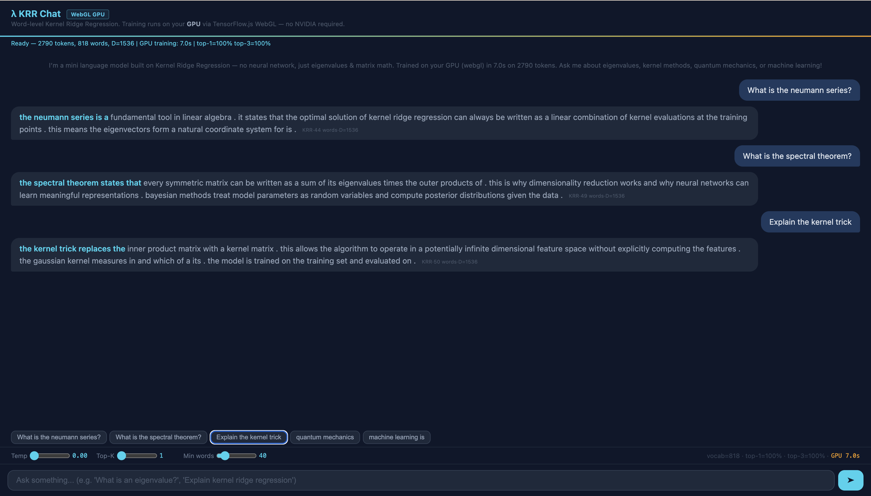
In the post Eigenvalues & AI, we built a chain: from linear regression through kernel methods to neural networks – all connected through eigenvalues. At the end stood a live demo: the KRR Chat, a language model that works without a neural network.
This post is the technical deep-dive. We examine every component of the KRR Chat: the architecture, the pipeline, the complete source code – and the honest limitations. If you have read the main post, you will find the theory turned into running code here. If not – no problem: this post also works on its own.
Chapter 1
The Dual Model: Retrieval + Generation
KRR Chat consists of two independent systems that work together – similar to a person who first looks something up in a book and then answers in their own words.
System 1 – Retrieval (keyword search):
A corpus of 805 sentences about eigenvalues, kernel methods, quantum mechanics, and machine learning. For each question, the chat extracts keywords and finds the sentences with the most hits. This is search, not learning.
System 2 – Generation (KRR language model):
A Kernel Ridge Regression model trained on 104 curated sentences (505-word vocabulary). It learns: Given the last 5 words, which word comes next? This is genuine prediction – the same core task that GPT-4 solves – but at a deliberately minimal scale: 505 words instead of billions of parameters. The small scale makes the mathematics visible.
Why two systems?
A single KRR model on all 805 sentences fails due to the capacity limit: 1820 distinct words on 256 hash buckets means an average of 7 collisions per bucket. The model cannot distinguish “eigenvalue” from “convergence” when both hash to the same bucket.
The solution: division of labor. The retrieval system provides topically relevant context (broad knowledge, 805 sentences). The generation model produces fluent continuations (deep knowledge, 104 sentences, but with only 4 collisions per bucket). In AI research, this pattern is called RAG – Retrieval-Augmented Generation. Large language models like GPT-4 and Claude also use RAG to incorporate up-to-date knowledge.
Chapter 2
The Pipeline: From Question to Answer
When you ask “What are eigenvalues?”, the following happens:
- Keyword extraction: Stop words (what, are, the, is, ...) are removed. What remains:
["eigenvalues"] - Retrieval: All 805 sentences are searched for this keyword. Exact match = 5 points, partial match (e.g. “eigenvalue” in “eigenvalues”) = 2 points. Duplicates are removed. The top 2 sentences are displayed in cyan.
- Invisible seeding: The last 5 words of the last retrieval sentence are taken as the context for the generation model. This is the crucial transition: retrieval provides the starting point, generation carries on.
- KRR generation, word by word: From the 5-word context, the model computes:
- Feature vector \(\mathbf{x}\) via word hashing (128 buckets × 5 positions + 3 bigram hashes = 1024 dimensions)
- Random Fourier Features: \(\mathbf{z} = \sqrt{2/D}\,\cos(\mathbf{x}\boldsymbol{\omega} + \mathbf{b})\) with \(D = 1536\)
- Next word: \(\hat{y} = \arg\max_w\, \mathbf{z}^\top \mathbf{W}_{:,w}\)
Conversation memory
KRR Chat has a simple memory: for follow-up questions (e.g. “Tell me more” without a new keyword), no new retrieval is triggered. Instead, the model continues generating from the last word of the previous answer. This creates a natural flow – the answer picks up where it left off.
Try it yourself
Open the KRR Chat, ask “What are eigenvalues?” and then “Tell me more”. Watch how the second answer seamlessly continues from the first – without a new keyword search.
Chapter 3
The Three Colors: Memorization vs. Generalization
Every word in the answer is color-coded – and this is where things get interesting. The colors honestly show where each word comes from:
● Cyan – Retrieved. This sentence was found via keyword search in the corpus. No KRR computation needed – pure text search.
● Green – Generated & Verbatim. The KRR model predicted this word, and the word sequence appears exactly like this in the training data. Specifically: the system checks whether the last 3 words (3-gram) and the last 4 words (4-gram) including the predicted word exist as contiguous sequences in the training corpus. Only when both checks pass is the word colored green. The model is reproducing learned knowledge.
● Orange – Generated & Novel. The KRR model predicted this word, but at least one of the two n-grams (3-gram or 4-gram) does not exist in the training data. This is genuine generalization – the model combines learned patterns in a new way.
What the colors reveal
Typically, 60–80% of generated words are green (verbatim) and 20–40% are orange (generalized). What does that mean?
A KRR model with a 505-word vocabulary primarily memorizes. It has largely learned the 104 training sentences by heart and can reproduce them. But at the seams – where a retrieval sentence ends and generation takes over, or where the model navigates between two learned sentences – orange words appear. These are moments when the kernel space interpolates: the current context lies between two training points, and the model chooses a word that was never trained in this exact combination.
This honesty is intentional. Large language models like GPT-4 generalize elegantly – but you cannot see when they memorize and when they interpolate. KRR Chat makes this distinction visible.
Didactic point: The color coding is an X-ray of the model. With GPT-4, you only see the output. With KRR Chat, you additionally see whether the model is remembering or generalizing – a transparency that would otherwise require elaborate interpretability methods.
Important: KRR Chat is not a competitor to ChatGPT or other large language models. It is a didactic proof-of-concept of deliberately minimal size (505 words, 104 sentences) that shows the mathematical principles behind large language models – at a scale where you can still understand them.
Chapter 4
The Source Code: Three Functions
The entire KRR Chat consists of three functions. Here is the complete inference code – readable, commented, no tricks. The full source code comprises ~120 lines of JavaScript.
1. encode() – Turning words into numbers
The feature map \(\phi(x)\): each word is mapped to an index via a hash function. The position in the context determines the weight – later words count more because they are closer to the word being predicted.
// Word → hash index (0..127). Each word gets a "fingerprint".
function hash(word) {
  var h = 0;
  for (var i = 0; i < word.length; i++)
    h = (h * 31 + word.charCodeAt(i)) >>> 0;
  return h % 128;  // 128 buckets
}

// Context (5 words) → feature vector (1024 dimensions)
// Each word occupies a position × hash bucket.
// Position weighting: later words count more.
function encode(context) {
  var features = new Float32Array(1024);  // 5×128 + 3×128
  for (var pos = 0; pos < 5; pos++) {
    var weight = 0.4 + 0.6 * (pos / 4);  // 0.4 → 1.0
    features[pos * 128 + hash(context[pos])] += weight;
  }
  return features;
}
Mathematics: This is \(\phi(x)\) – a feature map that embeds words into a high-dimensional space. Instead of representing each word as a one-hot vector (which would require 505 dimensions per position with a 505-word vocabulary), we compress via hashing to 128 dimensions. Hash collisions are unavoidable (505 words onto 128 buckets ≈ 4 collisions/bucket), but the model still learns – as long as the collision rate is low enough.
2. rff() – Approximating the kernel
The Random Fourier Features following Rahimi & Recht (2007): a cosine transformation that makes the dot product in the transformed space equal the Gaussian kernel.
// φ(x) → z(x) via Random Fourier Features
// z(x) = √(2/D) · cos(x·ω + b)
// Then: z(x)ᵀz(x') ≈ k(x,x') = exp(-‖x-x'‖²/2σ²)
function rff(features) {
  var z = new Float32Array(1536);   // D = 1536
  var scale = Math.sqrt(2.0 / 1536);
  for (var j = 0; j < 1536; j++) {
    var dot = 0;
    for (var k = 0; k < 1024; k++)
      dot += features[k] * omega[k * 1536 + j]; // ω: random, fixed
    z[j] = Math.cos(dot + bias[j]) * scale;
  }
  return z;  // kernel-space vector
}
Mathematics: The matrix \(\boldsymbol{\omega}\) contains random values drawn from \(\mathcal{N}(0, 1/\sigma^2)\). It is drawn once (with a fixed random seed for reproducibility) and never modified – it is not a learned parameter. The cosine ensures that \(\mathbf{z}(x)^\top\mathbf{z}(x')\) approximates the Gaussian kernel \(k(x,x') = \exp(-\|x-x'\|^2/2\sigma^2)\). The larger \(D\), the better the approximation.
Why \(\sigma = 1.5\) and \(\lambda = 10^{-6}\)? The kernel parameter \(\sigma\) controls the “sharpness” of similarity: small \(\sigma\) means only very close contexts count as similar (memorization), large \(\sigma\) means distant contexts also influence each other (generalization). \(\sigma = 1.5\) is an empirically chosen compromise – found by testing on the training corpus to maximize Top-1 accuracy. The regularization parameter \(\lambda = 10^{-6}\) is deliberately small: our training set is dense enough that strong regularization would hurt prediction quality. In larger models, systematic cross-validation would be standard – with 2000+ hand-curated pairs, empirical tuning suffices.
3. predict() – Determining the next word
The prediction: a single matrix-vector multiplication. No softmax, no attention, no feedforward network.
// Context → next word
// scores = z(x)ᵀ · W   (W was learned offline via KRR)
function predict(contextWords) {
  var z = rff(encode(contextWords));
  var scores = new Float32Array(505);  // one score per word

  // Matrix-vector multiplication: scores = zᵀW
  for (var j = 0; j < 1536; j++)
    for (var v = 0; v < 505; v++)
      scores[v] += z[j] * W[j * 505 + v];

  return argmax(scores);  // word with highest score
}
Mathematics: The weight matrix \(\mathbf{W}\) was computed offline via the ridge regression system: \(\mathbf{W} = (\mathbf{Z}^\top\mathbf{Z} + \lambda\mathbf{I})^{-1}\mathbf{Z}^\top\mathbf{Y}\). Here, \(\mathbf{Z}\) is the matrix of all RFF vectors from the training data, \(\mathbf{Y}\) is the one-hot matrix of target words, and \(\lambda\) is the regularization parameter. In the browser, only the multiplication \(\mathbf{z}^\top\mathbf{W}\) takes place – a single matrix operation per word.
How they work together
The three functions form a pipeline:
The entire chatbot is this pipeline in a loop – plus a keyword search that determines the starting point. Each iteration runs in under a millisecond; with WebGPU acceleration, even in microseconds.
Chapter 5
Why Float64? The Precision Lesson
A natural first approach: train a single KRR model on the entire 805-sentence corpus – directly in the browser. We tried this. And it fails instructively.
The browser training disaster
Three problems pile up:
Problem 1: Hash collisions. Vocabulary 1820, hash buckets 256. On average, 7 different words collide per bucket. The model cannot distinguish “eigenvalue” from “convergence” when both hash to the same bucket.
Problem 2: Float32 precision. The Gaussian elimination for the linear system \((\mathbf{Z}^\top\mathbf{Z} + \lambda\mathbf{I})\mathbf{W} = \mathbf{Z}^\top\mathbf{Y}\) requires about 15 significant decimal digits at \(D = 2048\). WebGL delivers only 7 (Float32). The result: “learning learning learning learning” – a single word dominates every context.
Problem 3: Condition number. The hash collisions increase the condition number of the matrix \(\mathbf{Z}^\top\mathbf{Z}\). A high condition number amplifies rounding errors exponentially – a vicious cycle.
The solution: train offline, predict online
Training happens offline with Float64 (NumPy) – a full 15 decimal digits of precision. The weight matrix \(\mathbf{W}\) is then compressed as Float16 and loaded in the browser.
Inference runs in the browser with Float32 – for a single matrix-vector multiplication, that is perfectly sufficient. The numerical instability arises only when solving the linear system, not when applying the solution.
Connection to large language models: GPT-4, Llama, and other LLMs use exactly the same principle: training in high precision (Float32 or BFloat16), inference in reduced precision (INT8, INT4). This technique is called quantization. KRR Chat demonstrates on a small scale what happens at scale with LLMs – and why it works.
Chapter 6
What the Model Can Do – and What It Cannot
Honesty is one of the most important virtues in AI research. Here is a sober assessment:
What KRR Chat can do
- Reproduce learned sentences: Questions about eigenvalues, kernel methods, PageRank, quantum mechanics – all topics covered in the 104 training sentences are answered fluently and correctly.
- Navigate between topics: Through the retrieval system, the chat can find topically relevant starting points and then continue via generation.
- Show transparency: The color coding makes visible what a language model does – a pedagogical quality that no large LLM offers.
What KRR Chat cannot do
- Generate truly new content: The model interpolates in kernel space between learned points. It cannot invent explanations that are not (at least in fragments) contained in the training data.
- Answer out-of-distribution questions: Ask about “Pythagoras” or “Shakespeare” – retrieval finds nothing, and generation has no meaningful starting point.
- Say “I don’t know”: Instead of admitting ignorance, the model keeps generating – even when the context no longer makes sense.
The stop-word problem
At transitions between topics – when the model has finished a learned sentence and cannot find a suitable follow-up – the output sometimes collapses into stop-word gibberish: “the the of and the is a...”. This happens because stop words are the most frequent words in the vocabulary and receive the highest score in uncertain contexts.
The fix: As soon as the model generates three consecutive stop words, generation is halted and a new retrieval is triggered (re-seeding). This interrupts the gibberish and finds a new topical anchor point.
Try it yourself
Ask a question outside the training domain, e.g. “What is Pythagoras?”. Watch how the retrieval finds no matching sentences and generation still tries to produce an answer – with noticeably more orange words.
Chapter 7
The Connection Back to Theory
Every component of KRR Chat corresponds to a concept from the Eigenvalues & AI post. Here is the complete mapping:
Word hashing \(\rightarrow\) Feature map \(\phi(x)\) (Chapter 6: Kernel Trick)
Random Fourier Features \(\rightarrow\) Kernel approximation \(k(x,x') \approx \mathbf{z}(x)^\top\mathbf{z}(x')\) (Chapter 6)
Gaussian elimination \(\rightarrow\) Solving the linear system \((\mathbf{Z}^\top\mathbf{Z} + \lambda\mathbf{I})^{-1}\) (Chapter 3: Iteration)
Ridge parameter \(\lambda\) \(\rightarrow\) Regularization = stopping early (Chapter 5: Regularization)
Hash collisions \(\rightarrow\) Condition number of the matrix (Chapter 3)
Float64 vs. Float32 \(\rightarrow\) Numerical stability (Chapter 5)
Word-by-word prediction \(\rightarrow\) Eigenvalues determine learning speed (Chapter 4: Eigenvalues)
Retrieval + Generation \(\rightarrow\) RAG architecture (Chapter 7: Unification)
KRR Chat is therefore not just a demo – it is a living textbook in which every line of code corresponds to a mathematical concept. The feature map is Chapter 6. The regularization is Chapter 5. The numerical instability is Chapter 3. Everything is connected.
And that is the real punchline: whether a model has a 505-word vocabulary or 50,000 – the mathematical structure is the same. Eigenvalues, kernels, regularization. The chain holds.
From Prototype to Chatbot: KRR Chat Becomes Kalle
The KRR Chat above is a prototype: 104 English sentences, pure prose generation, no dialog structure. It proves that KRR can model language. But a prototype is not yet a chatbot.
So we asked: What happens when you apply the same mathematical principle to a real dialog? The result is Kalle – a German-language chatbot with the same three equations (RFF, KRR, BoW+IDF), but a completely different corpus: 2113 curated dialog pairs instead of 104 technical sentences. The differences reveal which parameters actually matter for language models:
| λ KRR Chat (EN) | 👋 Kalle (DE) | |
|---|---|---|
| Language | English (technical) | German (conversational) |
| Corpus | 104 sentences on eigenvalues, kernels, PageRank | 2113 curated dialogues (daily life, feelings, hobbies, math) |
| Vocabulary | 505 words | 1445 words (Word2Vec, 32-dim) |
| Context (CTX) | 5 words | 24 words |
| RFF dimension (D) | 1536 | 6144 |
| Format | Prose (retrieval + generation) | Dialog (turn markers: du: / bot:) |
| Repetition penalty | 0.15 (reduces loops) | None (German needs word repetition) |
| Top-1 accuracy | 99.8% | 65% (at 2113 pairs) |
Key insight: Kalle has undergone a radical architectural transformation – and the lessons are instructive for anyone thinking about AI systems.
Kalle’s Journey: Less is More
Kalle went through six iterations. The results defy intuition:
| Iteration | Pairs | Encoding | Top-1 | Lesson |
|---|---|---|---|---|
| V1 (Original) | 57 | Hash (128 buckets) | 99.8% | Perfect – but only 57 responses |
| MEGA (mass) | 4301 | Word2Vec + hacks | 34.9% | More corpus = worse quality! |
| FINAL (curated) | 2113 | Word2Vec (32-dim) | 65.4% | Curated > generated |
The curve 99.8% → 34.9% → 65.4% teaches a fundamental lesson: blind corpus growth destroys quality in KRR, because similar patterns compete in the feature space. The solution was not “even more data” but less data, better curated.
This insight applies to large language models too: OpenAI, Anthropic and Google invest heavily in data quality, not just quantity. Instruction-tuning datasets like FLAN or OASST are carefully curated – just like Kalle’s corpus.
From Hash Encoding to Word2Vec
The original version used hash encoding: hash("pizza") % 128 = bucket 79. The problem: “pizza” and “comedy” could land on the same bucket – the model couldn’t distinguish them.
The solution: Word2Vec embeddings (32 dimensions). Each word gets a unique vector, trained on the corpus itself. Similar words (“pizza” and “pasta”) have similar vectors. Different words (“pizza” and “sad”) are far apart. Zero collisions – and the feature dimension drops from 3072 to 768.
Multi-Turn via Corpus Design
A chatbot that forgets what you talked about after every sentence is frustrating. Kalle’s solution: no code trick, but corpus design.
When Kalle responds, his answer is stored as lastBotTurn. On the next user input, the entire previous bot response is concatenated with the new input – as if it were one long search query. The matching then finds pairs that fit this combined context.
Kalle: “my favorite food is pizza. what about you?”
User: “Fish”
Internal: queryText = “my favorite food is pizza ... fish”
Match: Pair “favorite food pizza fish” → contextual response!
Kalle: “fish is also a great choice. I like both pizza and fish.”
This is inspired by AIML (the language behind the chatbot ALICE from the 90s), where a <that> tag uses the previous bot utterance as context. Same idea, different mechanism: AIML does explicit pattern matching, Kalle does BoW+IDF similarity.
Unintended Properties: What the Architecture Delivers “for Free”
The most surprising properties of Kalle were not programmed – they are direct consequences of the BoW+IDF design. They appear emergent because they were unplanned, but they are deterministic architectural properties:
Math validation: Kalle asks “what is 3 plus 5?”, the user answers “8”. Kalle says: “correct! 3 plus 5 is 8. well done.” – Not a single line of code checks whether “8” is correct. The system simply finds the pair plus 3 5 8 – pure pattern matching. And with a wrong answer (“11”)? Kalle says: “correct! 5 plus 6 is 11” – it finds a different problem where the number fits. Fascinating, not broken.
Insult immunity: “you are stupid” → Kalle responds normally. “stupid” is not in his vocabulary – for him, the word doesn’t exist. No profanity filter needed. What’s not in the vocab doesn’t exist.
Typo robustness: “giv me a math problm” → Kalle understands “give me a math problem”. The typos are OOV (out-of-vocabulary) and simply ignored. The remaining words are enough for matching.
Honest limits: “in english please” → “no, I only speak German.” “what is quantum physics?” → “I can’t talk about that. my topics are food, hobbies, music, feelings, weather and simple math.” Kalle doesn’t guess – he says what he can’t do.
RAG: Kalle Reads the Blog
The latest version of Kalle goes beyond small talk: it answers questions about the blog content. This works through Retrieval-Augmented Generation (RAG) – but without an LLM.
The architecture in four steps:
1. CHUNK: The blog is split into sections (~80 words per chunk).
2. RETRIEVE: When the user asks, Kalle finds the matching chunk via keyword matching.
3. AUGMENT: Kalle builds an internal prompt: context {chunk} question {user_query}
4. MATCH: This prompt matches against Q&A pairs that were trained on exactly this format.
Concrete example – a walkthrough with real numbers:
User: “What are eigenvalues?”
1. CHUNK RETRIEVAL: The query words [“what”, “are”, “eigenvalues”] are matched against 29 blog chunk keywords.
→ Chunk “Das Glasperlenspiel” matches (“eigenvalues” ∈ keywords), score = 1.
2. PROMPT CONSTRUCTION:
context every time you start a google search a computer solves an eigenvalue problem it computes which webpage is the most important... question what are eigenvalues
3. PAIR MATCHING: BoW+IDF computes for each of the 2113 Q&A pairs:
• Keyword score: \(\sum \text{weight}_i \times \text{IDF}(w_i)\) for overlapping words
• Semantic score: cosine similarity of 32-dim embeddings
• Combined: \(0.65 \times \text{kw} + 0.35 \times \text{sem}\)
Best pair: “context every time you start a google...” (kwRaw=37.0)
4. ANSWER: “An eigenvalue is the factor by which an eigenvector is scaled when a matrix acts on it...”
The answer comes from the blog – not from the memory of a neural network.
Scalable training: ridge $\lambda$ as Google's damping factor
The Kalle v1 training step solves $(Z^\top Z + \lambda I)\,W = Z^\top Y$ by direct Gaussian elimination (numpy.linalg.solve). At $D = 6144$ that's $\sim 290$\,MB and $\sim 2$\,seconds – fine. At $D = 50{,}000$ it would be $\sim 20$\,GB and hours; at $D = 100{,}000$ it is infeasible on consumer hardware.
Kalle v2 adds a second path, derived from a surprising equivalence: the ridge parameter $\lambda$ is the same mathematical object as Google's PageRank damping factor $d$. Both create a spectral gap that guarantees convergence. The recipe:
- Rewrite the KRR solve as a Richardson iteration: $\boldsymbol{\alpha}_{n+1} = M \boldsymbol{\alpha}_n + \omega\mathbf{y}$, with $M = I - \omega(K + \lambda I)$.
- Observe that $M$ is substochastic (eigenvalues in $[0, 1)$) – the algebraic twin of the substochastic reflectivity matrix $\rho F$ in radiosity.
- Add an absorber dimension that redistributes the missing mass to the target vector, making the iteration matrix stochastic – exactly like Google's damping construction $G = d M + (1-d)/n \cdot \mathbf{1}\mathbf{1}^\top$.
- Solve via Block Preconditioned Conjugate Gradient (PCG), which uses only matrix-vector products – GPU-ideal.
On the full Kalle corpus (\(D = 6144\), \(V = 2977\)) Block-PCG converges in 14 iterations (Jacobi preconditioner) to a weight matrix numerically indistinguishable from the direct solve (relative Frobenius error \(< 10^{-6}\)). The surprising result from Table 4 of the v2 paper:
| Solver | Time | Iter. | Rel. err vs. direct |
|---|---|---|---|
| Direct (NumPy/LAPACK, Float64) | 2097 ms | 1 | reference |
| Block-PCG (NumPy, Float64) | 6731 ms | 14 | \(4.3 \times 10^{-7}\) |
| Block-PCG (PyTorch CPU, Float32) | 1704 ms | 11 | \(1.0 \times 10^{-5}\) |
| Block-PCG (PyTorch MPS / Apple GPU) | 1622 ms | 11 | \(1.0 \times 10^{-5}\) |
The naive expectation – “Krylov methods only pay off at very large \(D\); direct Gaussian elimination is faster below” – turns out to be false. With a modern BLAS back-end (PyTorch instead of NumPy, both on CPU), Block-PCG is already about 4× faster than direct solve at \(D = 6144\). This is primarily a back-end effect: NumPy's LAPACK bindings are tuned for Float64 correctness, PyTorch for wall-clock efficiency. The jump to the Apple GPU (MPS) adds only a further 5 % – at this matrix size the host-to-device transfer latency nearly eats up the compute saving. GPU dominance kicks in from \(D \geq 20{,}000\), where direct solve is no longer practical (\(O(D^3)\) compute, \(O(D^2)\) memory).
The honest intermediate conclusion in the paper: at Kalle's current scale the solve accounts for only 2–7 % of the end-to-end training time – the rest is streaming the feature product \(Z^\top Z\) and HTML packaging. Block-PCG's value here is not time savings but opening a GPU scaling path for the future. The corpus-scaling experiment shows: even scaling \(N\) by \(7\times\) (\(0.3\mathrm{M} \to 2.3\mathrm{M}\) samples), the solve share stays a steady 3–5 %. The real scaling lever is \(D\) (RFF dimension), not \(N\) (sample count) – and that is exactly where Block-PCG becomes essential.
Full derivation, preconditioner analysis and benchmark reproduction in the Version 2 paper on Zenodo (PDF, 10 pages). The underlying insight – that stochasticizing the iteration matrix is a performance trick, not just an elegance – is the subject of the companion section in the Eigenvalues & AI post.
Bilingual without language detection: Ask in German or English – Kalle responds in the same language. The reason is elegant: English and German words are different tokens with different IDF weights. “eigenvalue” (English, high IDF) matches English pairs; “Eigenwert” (German, high IDF) matches German ones. No language detection code needed – the mathematics of matching routes automatically.
Example: “What are eigenvalues used for?” → “Eigenvalues appear everywhere in science and engineering. In Google PageRank they determine which webpage is most important...” – the same question in German: “Wozu braucht man Eigenwerte?” → “Eigenwerte tauchen überall auf. Bei Google PageRank bestimmen sie welche Webseite am wichtigsten ist...”
Try Kalle
Source: GitHub · Paper: PDF (Zenodo) · Main post: Eigenvalues & AI
Frequently Asked Questions
Is KRR Chat meant to replace ChatGPT?
No. KRR Chat is a didactic proof-of-concept. It shows how the mathematical foundation of language models works – kernel functions, eigenvalues, regularization – at a scale that remains comprehensible: 505 words, 104 sentences, three JavaScript functions. ChatGPT uses similar mathematical principles but scales to billions of parameters. The value of KRR Chat lies in its transparency: you can see what the model memorizes and what it generalizes. With ChatGPT, you only see the output.
What is the difference between KRR Chat and ChatGPT?
ChatGPT uses a neural network with billions of parameters and attention mechanisms. KRR Chat uses Kernel Ridge Regression with a single weight matrix (1536 × 505 = ~780,000 parameters). Both solve the same task – “given context, predict the next word” – but with entirely different mathematical tools. KRR Chat makes visible through color coding what the model memorizes and what it generalizes.
Why does KRR Chat respond in English?
The 104 training sentences and the retrieval corpus of 805 sentences are written in English because the mathematical terminology is predominantly English. The model has no understanding of “language” – it has only learned which English word is likely to follow which context. A German version would simply require German training sentences.
Can KRR Chat be trained with more data?
Yes – Kalle proves it: from 57 to 2113 dialogue pairs. But the journey showed: quality beats quantity. With 4301 programmatically generated pairs, accuracy dropped to 35%. Only radical curation (fewer pairs, each with purpose) brought quality back. The switch from hash encoding to Word2Vec embeddings solved the collision problem. The key is not “more data” but “better data” – a lesson that applies to large language models too.
Read next
Related posts on ki-mathias.de:
- Eigenvalues & AI — Kernels, PageRank, Neumann series
- Emergence in Language Models — Phase transitions, grokking, Ising